Reading in data locally and from the web
Contents
Reading in data locally and from the web
We need to import the pandas package in order to read data into Python
import pandas as pd
import warnings
warnings.filterwarnings('ignore')
Overview
In this chapter, you’ll learn to read tabular data of various formats into Python from your local device (e.g., your laptop) and the web. “Reading” (or “loading”) \index{loading|see{reading}}\index{reading!definition} is the process of converting data (stored as plain text, a database, HTML, etc.) into an object (e.g., a data frame) that Python can easily access and manipulate. Thus reading data is the gateway to any data analysis; you won’t be able to analyze data unless you’ve loaded it first. And because there are many ways to store data, there are similarly many ways to read data into Python. The more time you spend upfront matching the data reading method to the type of data you have, the less time you will have to devote to re-formatting, cleaning and wrangling your data (the second step to all data analyses). It’s like making sure your shoelaces are tied well before going for a run so that you don’t trip later on!
Chapter learning objectives
By the end of the chapter, readers will be able to do the following:
Define the following:
absolute file path
relative file path
Uniform Resource Locator (URL)
Read data into Python using an absolute path, relative path and a URL.
Compare and contrast the following functions:
read_csvread_tableread_excel
Match the following
pandas.read_*function arguments to their descriptions:filepath_or_buffersepnamesskiprows
Choose the appropriate
pandas.read_*function and function arguments to load a given plain text tabular data set into Python.Use
pandaspackage’sread_excelfunction and arguments to load a sheet from an excel file into Python.Connect to a database using the
SQLAlchemylibrary.List the tables in a database using
SQLAlchemylibrary’stable_namesfunctionCreate a reference to a database table that is queriable using the
SQLAlchemylibrary’sselectandwherefunctionsUse
.to_csvto save a data frame to a csv file(Optional) Obtain data using application programming interfaces (APIs) and web scraping.
Read/scrape data from an internet URL using the
BeautifulSouppackageCompare downloading tabular data from a plain text file (e.g. *.csv) from the web versus scraping data from a .html file
Absolute and relative file paths
This chapter will discuss the different functions we can use to import data into Python, but before we can talk about how we read the data into Python with these functions, we first need to talk about where the data lives. When you load a data set into Python, you first need to tell Python where those files live. The file could live on your computer (local) \index{location|see{path}} \index{path!local, remote, relative, absolute} or somewhere on the internet (remote).
The place where the file lives on your computer is called the “path”. You can think of the path as directions to the file. There are two kinds of paths: relative paths and absolute paths. A relative path is where the file is with respect to where you currently are on the computer (e.g., where the file you’re working in is). On the other hand, an absolute path is where the file is in respect to the computer’s filesystem base (or root) folder.
Suppose our computer’s filesystem looks like the picture in
Fig. 9, and we are working in a
file titled worksheet_02.ipynb. If we want to
read the .csv file named happiness_report.csv into Python, we could do this
using either a relative or an absolute path. We show both choices
below.\index{Happiness Report}
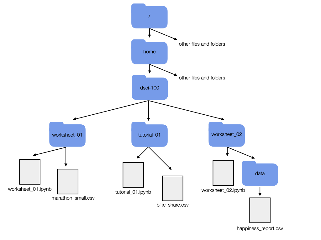
Fig. 9 Example file system
Reading happiness_report.csv using a relative path:
happy_data = pd.read_csv("data/happiness_report.csv")
Reading happiness_report.csv using an absolute path:
happy_data = pd.read_csv("/home/dsci-100/worksheet_02/data/happiness_report.csv")
So which one should you use? Generally speaking, to ensure your code can be run
on a different computer, you should use relative paths. An added bonus is that
it’s also less typing! Generally, you should use relative paths because the file’s
absolute path (the names of
folders between the computer’s root / and the file) isn’t usually the same
across different computers. For example, suppose Fatima and Jayden are working on a
project together on the happiness_report.csv data. Fatima’s file is stored at
/home/Fatima/project/data/happiness_report.csv,
while Jayden’s is stored at
/home/Jayden/project/data/happiness_report.csv.
Even though Fatima and Jayden stored their files in the same place on their
computers (in their home folders), the absolute paths are different due to
their different usernames. If Jayden has code that loads the
happiness_report.csv data using an absolute path, the code won’t work on
Fatima’s computer. But the relative path from inside the project folder
(data/happiness_report.csv) is the same on both computers; any code that uses
relative paths will work on both!
Your file could be stored locally, as we discussed, or it could also be somewhere on the internet (remotely). A Uniform Resource Locator (URL) (web address) \index{URL} indicates the location of a resource on the internet and helps us retrieve that resource. Next, we will discuss how to get either locally or remotely stored data into Python.
Reading tabular data from a plain text file into Python
read_csv to read in comma-separated files {#readcsv}
Now that we have learned about where data could be, we will learn about how
to import data into Python using various functions. Specifically, we will learn how
to read tabular data from a plain text file (a document containing only text)
into Python and write tabular data to a file out of Python. The function we use to do this
depends on the file’s format. For example, in the last chapter, we learned about using
the pandas read_csv function when reading .csv (comma-separated values)
files. \index{csv} In that case, the separator or delimiter \index{reading!delimiter} that divided our columns was a
comma (,). We only learned the case where the data matched the expected defaults
of the read_csv function \index{read function!read_csv}
(column names are present, and commas are used as the delimiter between columns).
In this section, we will learn how to read
files that do not satisfy the default expectations of read_csv.
Before we jump into the cases where the data aren’t in the expected default format
for pandas and read_csv, let’s revisit the more straightforward
case where the defaults hold, and the only argument we need to give to the function
is the path to the file, data/can_lang.csv. The can_lang data set contains
language data from the 2016 Canadian census. \index{Canadian languages!canlang data}
We put data/ before the file’s
name when we are loading the data set because this data set is located in a
sub-folder, named data, relative to where we are running our Python code.
Here is what the file would look like in a plain text editor (a program that removes all formatting, like bolding or different fonts):
category,language,mother_tongue,most_at_home,most_at_work,lang_known
Aboriginal languages,"Aboriginal languages, n.o.s.",590,235,30,665
Non-Official & Non-Aboriginal languages,Afrikaans,10260,4785,85,23415
Non-Official & Non-Aboriginal languages,"Afro-Asiatic languages, n.i.e.",1150,44
Non-Official & Non-Aboriginal languages,Akan (Twi),13460,5985,25,22150
Non-Official & Non-Aboriginal languages,Albanian,26895,13135,345,31930
Aboriginal languages,"Algonquian languages, n.i.e.",45,10,0,120
Aboriginal languages,Algonquin,1260,370,40,2480
Non-Official & Non-Aboriginal languages,American Sign Language,2685,3020,1145,21
Non-Official & Non-Aboriginal languages,Amharic,22465,12785,200,33670
And here is a review of how we can use read_csv to load it into Python. First we
load the pandas \index{tidyverse} package to gain access to useful
functions for reading the data.
Next we use read_csv to load the data into Python, and in that call we specify the
relative path to the file.
canlang_data = pd.read_csv("data/can_lang.csv")
canlang_data
| category | language | mother_tongue | most_at_home | most_at_work | lang_known | |
|---|---|---|---|---|---|---|
| 0 | Aboriginal languages | Aboriginal languages, n.o.s. | 590 | 235 | 30 | 665 |
| 1 | Non-Official & Non-Aboriginal languages | Afrikaans | 10260 | 4785 | 85 | 23415 |
| 2 | Non-Official & Non-Aboriginal languages | Afro-Asiatic languages, n.i.e. | 1150 | 445 | 10 | 2775 |
| 3 | Non-Official & Non-Aboriginal languages | Akan (Twi) | 13460 | 5985 | 25 | 22150 |
| 4 | Non-Official & Non-Aboriginal languages | Albanian | 26895 | 13135 | 345 | 31930 |
| ... | ... | ... | ... | ... | ... | ... |
| 209 | Non-Official & Non-Aboriginal languages | Wolof | 3990 | 1385 | 10 | 8240 |
| 210 | Aboriginal languages | Woods Cree | 1840 | 800 | 75 | 2665 |
| 211 | Non-Official & Non-Aboriginal languages | Wu (Shanghainese) | 12915 | 7650 | 105 | 16530 |
| 212 | Non-Official & Non-Aboriginal languages | Yiddish | 13555 | 7085 | 895 | 20985 |
| 213 | Non-Official & Non-Aboriginal languages | Yoruba | 9080 | 2615 | 15 | 22415 |
214 rows × 6 columns
Skipping rows when reading in data
Oftentimes, information about how data was collected, or other relevant information, is included at the top of the data file. This information is usually written in sentence and paragraph form, with no delimiter because it is not organized into columns. An example of this is shown below. This information gives the data scientist useful context and information about the data, however, it is not well formatted or intended to be read into a data frame cell along with the tabular data that follows later in the file.
Data source: https://ttimbers.github.io/canlang/
Data originally published in: Statistics Canada Census of Population 2016.
Reproduced and distributed on an as-is basis with their permission.
category,language,mother_tongue,most_at_home,most_at_work,lang_known
Aboriginal languages,"Aboriginal languages, n.o.s.",590,235,30,665
Non-Official & Non-Aboriginal languages,Afrikaans,10260,4785,85,23415
Non-Official & Non-Aboriginal languages,"Afro-Asiatic languages, n.i.e.",1150,44
Non-Official & Non-Aboriginal languages,Akan (Twi),13460,5985,25,22150
Non-Official & Non-Aboriginal languages,Albanian,26895,13135,345,31930
Aboriginal languages,"Algonquian languages, n.i.e.",45,10,0,120
Aboriginal languages,Algonquin,1260,370,40,2480
Non-Official & Non-Aboriginal languages,American Sign Language,2685,3020,1145,21
Non-Official & Non-Aboriginal languages,Amharic,22465,12785,200,33670
With this extra information being present at the top of the file, using
read_csv as we did previously does not allow us to correctly load the data
into Python. In the case of this file we end up only reading in one column of the
data set:
canlang_data = pd.read_csv("data/can_lang-meta-data.csv")
ParserError: Error tokenizing data. C error: Expected 3 fields in line 3, saw 6
Note: In contrast to the normal and expected messages above, this time Python printed out a Parsing error for us indicating that there might be a problem with how our data is being read in. \index{warning}
To successfully read data like this into Python, the skiprows
argument \index{read function!skip argument} can be useful to tell Python
how many lines to skip before
it should start reading in the data. In the example above, we would set this
value to 2 and pass header as None to read and load the data correctly.
canlang_data = pd.read_csv("data/can_lang-meta-data.csv", skiprows=2, header=None)
canlang_data
| 0 | 1 | 2 | 3 | 4 | 5 | |
|---|---|---|---|---|---|---|
| 0 | Aboriginal languages | Aboriginal languages, n.o.s. | 590 | 235 | 30 | 665 |
| 1 | Non-Official & Non-Aboriginal languages | Afrikaans | 10260 | 4785 | 85 | 23415 |
| 2 | Non-Official & Non-Aboriginal languages | Afro-Asiatic languages, n.i.e. | 1150 | 445 | 10 | 2775 |
| 3 | Non-Official & Non-Aboriginal languages | Akan (Twi) | 13460 | 5985 | 25 | 22150 |
| 4 | Non-Official & Non-Aboriginal languages | Albanian | 26895 | 13135 | 345 | 31930 |
| ... | ... | ... | ... | ... | ... | ... |
| 423 | Non-Official & Non-Aboriginal languages | Wolof | 3990 | 1385 | 10 | 8240 |
| 424 | Aboriginal languages | Woods Cree | 1840 | 800 | 75 | 2665 |
| 425 | Non-Official & Non-Aboriginal languages | Wu (Shanghainese) | 12915 | 7650 | 105 | 16530 |
| 426 | Non-Official & Non-Aboriginal languages | Yiddish | 13555 | 7085 | 895 | 20985 |
| 427 | Non-Official & Non-Aboriginal languages | Yoruba | 9080 | 2615 | 15 | 22415 |
428 rows × 6 columns
How did we know to skip two lines? We looked at the data! The first two lines of the data had information we didn’t need to import:
Source: Statistics Canada, Census of Population, 2016. Reproduced and distributed on an "as is" basis with the permission of Statistics Canada.
Date collected: 2020/07/09
The column names began at line 3, so we skipped the first two lines.
read_csv with sep argument to read in tab-separated files
Another common way data is stored is with tabs as the delimiter. Notice the
data file, can_lang.tsv, has tabs in between the columns instead of
commas.
category    language    mother_tongue   most_at_home    most_at_work    lang_kno
Aboriginal languages    Aboriginal languages, n.o.s.    590 235 30  665
Non-Official & Non-Aboriginal languages Afrikaans   10260   4785    85  23415
Non-Official & Non-Aboriginal languages Afro-Asiatic languages, n.i.e.  1150
Non-Official & Non-Aboriginal languages Akan (Twi)  13460   5985    25  22150
Non-Official & Non-Aboriginal languages Albanian    26895   13135   345 31930
Aboriginal languages    Algonquian languages, n.i.e.    45  10  0   120
Aboriginal languages    Algonquin   1260    370 40  2480
Non-Official & Non-Aboriginal languages American Sign Language  2685    3020
Non-Official & Non-Aboriginal languages Amharic 22465   12785   200 33670
To read in this type of data, we can use the read_csv with sep argument
\index{tab-separated values|see{tsv}}\index{tsv}\index{read function!read_tsv}
to read in .tsv (tab separated values) files.
canlang_data = pd.read_csv("data/can_lang.tsv", sep="\t", header=None)
canlang_data
| 0 | 1 | 2 | 3 | 4 | 5 | |
|---|---|---|---|---|---|---|
| 0 | Aboriginal languages | Aboriginal languages, n.o.s. | 590 | 235 | 30 | 665 |
| 1 | Non-Official & Non-Aboriginal languages | Afrikaans | 10260 | 4785 | 85 | 23415 |
| 2 | Non-Official & Non-Aboriginal languages | Afro-Asiatic languages, n.i.e. | 1150 | 445 | 10 | 2775 |
| 3 | Non-Official & Non-Aboriginal languages | Akan (Twi) | 13460 | 5985 | 25 | 22150 |
| 4 | Non-Official & Non-Aboriginal languages | Albanian | 26895 | 13135 | 345 | 31930 |
| ... | ... | ... | ... | ... | ... | ... |
| 209 | Non-Official & Non-Aboriginal languages | Wolof | 3990 | 1385 | 10 | 8240 |
| 210 | Aboriginal languages | Woods Cree | 1840 | 800 | 75 | 2665 |
| 211 | Non-Official & Non-Aboriginal languages | Wu (Shanghainese) | 12915 | 7650 | 105 | 16530 |
| 212 | Non-Official & Non-Aboriginal languages | Yiddish | 13555 | 7085 | 895 | 20985 |
| 213 | Non-Official & Non-Aboriginal languages | Yoruba | 9080 | 2615 | 15 | 22415 |
214 rows × 6 columns
Let’s compare the data frame here to the resulting data frame in Section
@ref(readcsv) after using read_csv. Notice anything? They look the same! The
same number of columns/rows and column names! So we needed to use different
tools for the job depending on the file format and our resulting table
(canlang_data) in both cases was the same!
read_table as a more flexible method to get tabular data into Python
read_csv and read_csv with argument sep are actually just special cases of the more general
read_table \index{read function!read_delim} function. We can use
read_table to import both comma and tab-separated files (and more), we just
have to specify the delimiter. The can_lang.tsv is a different version of
this same data set with no column names and uses tabs as the delimiter
\index{reading!delimiter} instead of commas.
Here is how the file would look in a plain text editor:
Aboriginal languages    Aboriginal languages, n.o.s.    590 235 30  665
Non-Official & Non-Aboriginal languages Afrikaans   10260   4785    85  23415
Non-Official & Non-Aboriginal languages Afro-Asiatic languages, n.i.e.  1150
Non-Official & Non-Aboriginal languages Akan (Twi)  13460   5985    25  22150
Non-Official & Non-Aboriginal languages Albanian    26895   13135   345 31930
Aboriginal languages    Algonquian languages, n.i.e.    45  10  0   120
Aboriginal languages    Algonquin   1260    370 40  2480
Non-Official & Non-Aboriginal languages American Sign Language  2685    3020
Non-Official & Non-Aboriginal languages Amharic 22465   12785   200 33670
Non-Official & Non-Aboriginal languages Arabic  419890  223535  5585    629055
To get this into Python using the read_table function, we specify the first
argument as the path to the file (as done with read_csv), and then provide
values to the sep \index{read function!delim argument} argument (here a
tab, which we represent by "\t").
Note:
\tis an example of an escaped character, which always starts with a backslash (\). \index{escape character} Escaped characters are used to represent non-printing characters (like the tab) or characters with special meanings (such as quotation marks).
canlang_data =  pd.read_csv("data/can_lang.tsv",
                           sep = "\t",
                           header = None)
canlang_data
| 0 | 1 | 2 | 3 | 4 | 5 | |
|---|---|---|---|---|---|---|
| 0 | Aboriginal languages | Aboriginal languages, n.o.s. | 590 | 235 | 30 | 665 |
| 1 | Non-Official & Non-Aboriginal languages | Afrikaans | 10260 | 4785 | 85 | 23415 |
| 2 | Non-Official & Non-Aboriginal languages | Afro-Asiatic languages, n.i.e. | 1150 | 445 | 10 | 2775 |
| 3 | Non-Official & Non-Aboriginal languages | Akan (Twi) | 13460 | 5985 | 25 | 22150 |
| 4 | Non-Official & Non-Aboriginal languages | Albanian | 26895 | 13135 | 345 | 31930 |
| ... | ... | ... | ... | ... | ... | ... |
| 209 | Non-Official & Non-Aboriginal languages | Wolof | 3990 | 1385 | 10 | 8240 |
| 210 | Aboriginal languages | Woods Cree | 1840 | 800 | 75 | 2665 |
| 211 | Non-Official & Non-Aboriginal languages | Wu (Shanghainese) | 12915 | 7650 | 105 | 16530 |
| 212 | Non-Official & Non-Aboriginal languages | Yiddish | 13555 | 7085 | 895 | 20985 |
| 213 | Non-Official & Non-Aboriginal languages | Yoruba | 9080 | 2615 | 15 | 22415 |
214 rows × 6 columns
Data frames in Python need to have column names. Thus if you read in data that
don’t have column names, Python will assign names automatically. In the example
above, Python assigns each column a name of 0, 1, 2, 3, 4, 5.
It is best to rename your columns to help differentiate between them
(e.g., 0, 1, etc., are not very descriptive names and will make it more confusing as
you code). To rename your columns, you can use the rename function
\index{rename} from the pandas package.
The argument of the rename function is columns, which is a dictionary,
where the keys are the old column names and values are the new column names.
We rename the old 0, 1, ..., 5
columns in the canlang_data data frame to more descriptive names below, with the
inplace argument as True, so that the columns are renamed in place.
canlang_data.rename(columns = {0:'category',
                               1:'language',
                               2:'mother_tongue',
                               3:'most_at_home',
                               4:'most_at_work',
                               5:'lang_known'}, inplace = True)


canlang_data
| category | language | mother_tongue | most_at_home | most_at_work | lang_known | |
|---|---|---|---|---|---|---|
| 0 | Aboriginal languages | Aboriginal languages, n.o.s. | 590 | 235 | 30 | 665 |
| 1 | Non-Official & Non-Aboriginal languages | Afrikaans | 10260 | 4785 | 85 | 23415 |
| 2 | Non-Official & Non-Aboriginal languages | Afro-Asiatic languages, n.i.e. | 1150 | 445 | 10 | 2775 |
| 3 | Non-Official & Non-Aboriginal languages | Akan (Twi) | 13460 | 5985 | 25 | 22150 |
| 4 | Non-Official & Non-Aboriginal languages | Albanian | 26895 | 13135 | 345 | 31930 |
| ... | ... | ... | ... | ... | ... | ... |
| 209 | Non-Official & Non-Aboriginal languages | Wolof | 3990 | 1385 | 10 | 8240 |
| 210 | Aboriginal languages | Woods Cree | 1840 | 800 | 75 | 2665 |
| 211 | Non-Official & Non-Aboriginal languages | Wu (Shanghainese) | 12915 | 7650 | 105 | 16530 |
| 212 | Non-Official & Non-Aboriginal languages | Yiddish | 13555 | 7085 | 895 | 20985 |
| 213 | Non-Official & Non-Aboriginal languages | Yoruba | 9080 | 2615 | 15 | 22415 |
214 rows × 6 columns
The column names can also be assigned to the dataframe while reading it from the file by passing a
list of column names to the names argument. read_csv and read_table have a names argument,
\index{read function!col_names argument} whose default value is [].
canlang_data =  pd.read_csv("data/can_lang.tsv",
                           sep = "\t",
                           header = None,
                           names = ['category', 'language', 'mother_tongue', 'most_at_home', 'most_at_work', 'lang_known'])
canlang_data
| category | language | mother_tongue | most_at_home | most_at_work | lang_known | |
|---|---|---|---|---|---|---|
| 0 | Aboriginal languages | Aboriginal languages, n.o.s. | 590 | 235 | 30 | 665 |
| 1 | Non-Official & Non-Aboriginal languages | Afrikaans | 10260 | 4785 | 85 | 23415 |
| 2 | Non-Official & Non-Aboriginal languages | Afro-Asiatic languages, n.i.e. | 1150 | 445 | 10 | 2775 |
| 3 | Non-Official & Non-Aboriginal languages | Akan (Twi) | 13460 | 5985 | 25 | 22150 |
| 4 | Non-Official & Non-Aboriginal languages | Albanian | 26895 | 13135 | 345 | 31930 |
| ... | ... | ... | ... | ... | ... | ... |
| 209 | Non-Official & Non-Aboriginal languages | Wolof | 3990 | 1385 | 10 | 8240 |
| 210 | Aboriginal languages | Woods Cree | 1840 | 800 | 75 | 2665 |
| 211 | Non-Official & Non-Aboriginal languages | Wu (Shanghainese) | 12915 | 7650 | 105 | 16530 |
| 212 | Non-Official & Non-Aboriginal languages | Yiddish | 13555 | 7085 | 895 | 20985 |
| 213 | Non-Official & Non-Aboriginal languages | Yoruba | 9080 | 2615 | 15 | 22415 |
214 rows × 6 columns
Reading tabular data directly from a URL
We can also use read_csv, read_table(and related functions)
to read in data directly from a Uniform Resource Locator (URL) that
contains tabular data. \index{URL!reading from} Here, we provide the URL to
read_* as the path to the file instead of a path to a local file on our
computer. We need to surround the URL with quotes similar to when we specify a
path on our local computer. All other arguments that we use are the same as
when using these functions with a local file on our computer.
url = "https://raw.githubusercontent.com/UBC-DSCI/introduction-to-datascience-python/reading/source/data/can_lang.csv"
pd.read_csv(url)
canlang_data = pd.read_csv(url)

canlang_data
| category | language | mother_tongue | most_at_home | most_at_work | lang_known | |
|---|---|---|---|---|---|---|
| 0 | Aboriginal languages | Aboriginal languages, n.o.s. | 590 | 235 | 30 | 665 |
| 1 | Non-Official & Non-Aboriginal languages | Afrikaans | 10260 | 4785 | 85 | 23415 |
| 2 | Non-Official & Non-Aboriginal languages | Afro-Asiatic languages, n.i.e. | 1150 | 445 | 10 | 2775 |
| 3 | Non-Official & Non-Aboriginal languages | Akan (Twi) | 13460 | 5985 | 25 | 22150 |
| 4 | Non-Official & Non-Aboriginal languages | Albanian | 26895 | 13135 | 345 | 31930 |
| ... | ... | ... | ... | ... | ... | ... |
| 209 | Non-Official & Non-Aboriginal languages | Wolof | 3990 | 1385 | 10 | 8240 |
| 210 | Aboriginal languages | Woods Cree | 1840 | 800 | 75 | 2665 |
| 211 | Non-Official & Non-Aboriginal languages | Wu (Shanghainese) | 12915 | 7650 | 105 | 16530 |
| 212 | Non-Official & Non-Aboriginal languages | Yiddish | 13555 | 7085 | 895 | 20985 |
| 213 | Non-Official & Non-Aboriginal languages | Yoruba | 9080 | 2615 | 15 | 22415 |
214 rows × 6 columns
Previewing a data file before reading it into Python
In all the examples above, we gave you previews of the data file before we read it into Python. Previewing data is essential to see whether or not there are column names, what the delimiters are, and if there are lines you need to skip. You should do this yourself when trying to read in data files. You can preview files in a plain text editor by right-clicking on the file, selecting “Open With,” and choosing a plain text editor (e.g., Notepad).
Reading tabular data from a Microsoft Excel file
There are many other ways to store tabular data sets beyond plain text files,
and similarly, many ways to load those data sets into Python. For example, it is
very common to encounter, and need to load into Python, data stored as a Microsoft
Excel \index{Excel spreadsheet}\index{Microsoft Excel|see{Excel
spreadsheet}}\index{xlsx|see{Excel spreadsheet}} spreadsheet (with the file name
extension .xlsx). To be able to do this, a key thing to know is that even
though .csv and .xlsx files look almost identical when loaded into Excel,
the data themselves are stored completely differently. While .csv files are
plain text files, where the characters you see when you open the file in a text
editor are exactly the data they represent, this is not the case for .xlsx
files. Take a look at a snippet of what a .xlsx file would look like in a text editor:
,?'O
    _rels/.rels???J1??>E?{7?
<?V????w8?'J???'QrJ???Tf?d??d?o?wZ'???@>?4'?|??hlIo??F
t                                                       8f??3wn
????t??u"/
          %~Ed2??<?w??
                       ?Pd(??J-?E???7?'t(?-GZ?????y???c~N?g[^_r?4
                                                                  yG?O
                                                                      ?K??G?


     ]TUEe??O??c[???????6q??s??d?m???\???H?^????3} ?rZY? ?:L60?^?????XTP+?|?
X?a??4VT?,D?Jq
This type of file representation allows Excel files to store additional things
that you cannot store in a .csv file, such as fonts, text formatting,
graphics, multiple sheets and more. And despite looking odd in a plain text
editor, we can read Excel spreadsheets into Python using the pandas package’s read_excel
function developed specifically for this
purpose. \index{readxl}\index{read function!read_excel}
canlang_data = pd.read_excel("data/can_lang.xlsx")
canlang_data
---------------------------------------------------------------------------
ModuleNotFoundError                       Traceback (most recent call last)
File /opt/miniconda3/envs/dsci100/lib/python3.9/site-packages/pandas/compat/_optional.py:138, in import_optional_dependency(name, extra, errors, min_version)
    137 try:
--> 138     module = importlib.import_module(name)
    139 except ImportError:

File /opt/miniconda3/envs/dsci100/lib/python3.9/importlib/__init__.py:127, in import_module(name, package)
    126         level += 1
--> 127 return _bootstrap._gcd_import(name[level:], package, level)

File <frozen importlib._bootstrap>:1030, in _gcd_import(name, package, level)

File <frozen importlib._bootstrap>:1007, in _find_and_load(name, import_)

File <frozen importlib._bootstrap>:984, in _find_and_load_unlocked(name, import_)

ModuleNotFoundError: No module named 'openpyxl'

During handling of the above exception, another exception occurred:

ImportError                               Traceback (most recent call last)
Input In [11], in <cell line: 1>()
----> 1 canlang_data = pd.read_excel("data/can_lang.xlsx")
      2 canlang_data

File /opt/miniconda3/envs/dsci100/lib/python3.9/site-packages/pandas/util/_decorators.py:311, in deprecate_nonkeyword_arguments.<locals>.decorate.<locals>.wrapper(*args, **kwargs)
    305 if len(args) > num_allow_args:
    306     warnings.warn(
    307         msg.format(arguments=arguments),
    308         FutureWarning,
    309         stacklevel=stacklevel,
    310     )
--> 311 return func(*args, **kwargs)

File /opt/miniconda3/envs/dsci100/lib/python3.9/site-packages/pandas/io/excel/_base.py:457, in read_excel(io, sheet_name, header, names, index_col, usecols, squeeze, dtype, engine, converters, true_values, false_values, skiprows, nrows, na_values, keep_default_na, na_filter, verbose, parse_dates, date_parser, thousands, decimal, comment, skipfooter, convert_float, mangle_dupe_cols, storage_options)
    455 if not isinstance(io, ExcelFile):
    456     should_close = True
--> 457     io = ExcelFile(io, storage_options=storage_options, engine=engine)
    458 elif engine and engine != io.engine:
    459     raise ValueError(
    460         "Engine should not be specified when passing "
    461         "an ExcelFile - ExcelFile already has the engine set"
    462     )

File /opt/miniconda3/envs/dsci100/lib/python3.9/site-packages/pandas/io/excel/_base.py:1419, in ExcelFile.__init__(self, path_or_buffer, engine, storage_options)
   1416 self.engine = engine
   1417 self.storage_options = storage_options
-> 1419 self._reader = self._engines[engine](self._io, storage_options=storage_options)

File /opt/miniconda3/envs/dsci100/lib/python3.9/site-packages/pandas/io/excel/_openpyxl.py:524, in OpenpyxlReader.__init__(self, filepath_or_buffer, storage_options)
    509 def __init__(
    510     self,
    511     filepath_or_buffer: FilePath | ReadBuffer[bytes],
    512     storage_options: StorageOptions = None,
    513 ) -> None:
    514     """
    515     Reader using openpyxl engine.
    516
   (...)
    522         passed to fsspec for appropriate URLs (see ``_get_filepath_or_buffer``)
    523     """
--> 524     import_optional_dependency("openpyxl")
    525     super().__init__(filepath_or_buffer, storage_options=storage_options)

File /opt/miniconda3/envs/dsci100/lib/python3.9/site-packages/pandas/compat/_optional.py:141, in import_optional_dependency(name, extra, errors, min_version)
    139 except ImportError:
    140     if errors == "raise":
--> 141         raise ImportError(msg)
    142     else:
    143         return None

ImportError: Missing optional dependency 'openpyxl'.  Use pip or conda to install openpyxl.
If the .xlsx file has multiple sheets, you have to use the sheet_name argument
to specify the sheet number or name. You can also specify cell ranges using the
usecols argument(Example: usecols="A:D" for including cells from A to D).
This functionality is useful when a single sheet contains
multiple tables (a sad thing that happens to many Excel spreadsheets since this
makes reading in data more difficult).
As with plain text files, you should always explore the data file before importing it into Python. Exploring the data beforehand helps you decide which arguments you need to load the data into Python successfully. If you do not have the Excel program on your computer, you can use other programs to preview the file. Examples include Google Sheets and Libre Office.
In Table 2 we summarize the read_* functions we covered
in this chapter. We also include the read_csv2 function for data separated by
semicolons ;, which you may run into with data sets where the decimal is
represented by a comma instead of a period (as with some data sets from
European countries).
Data File Type |
Python Function |
Python Package |
|---|---|---|
Comma ( |
|
|
Tab ( |
|
|
Semicolon ( |
|
|
Various formats ( |
|
|
Excel files ( |
|
|
Reading data from a database
Another very common form of data storage is the relational database. Databases \index{database} are great when you have large data sets or multiple users working on a project. There are many relational database management systems, such as SQLite, MySQL, PostgreSQL, Oracle, and many more. These different relational database management systems each have their own advantages and limitations. Almost all employ SQL (structured query language) to obtain data from the database. But you don’t need to know SQL to analyze data from a database; several packages have been written that allow you to connect to relational databases and use the Python programming language to obtain data. In this book, we will give examples of how to do this using Python with SQLite and PostgreSQL databases.
Reading data from a SQLite database
SQLite \index{database!SQLite} is probably the simplest relational database system
that one can use in combination with Python. SQLite databases are self-contained and
usually stored and accessed locally on one computer. Data is usually stored in
a file with a .db extension. Similar to Excel files, these are not plain text
files and cannot be read in a plain text editor.
The first thing you need to do to read data into Python from a database is to
connect to the database. We do that using the create_engine function from the
sal (SQLAlchemy) package. \index{database!connect} This does not read
in the data, but simply tells Python where the database is and opens up a
communication channel that Python can use to send SQL commands to the database.
import sqlalchemy as sal
from sqlalchemy import create_engine, select, MetaData, Table


db = sal.create_engine("sqlite:///data/can_lang.db")
conn = db.connect()
Often relational databases have many tables; thus, in order to retrieve
data from a database, you need to know the name of the table
in which the data is stored. You can get the names of
all the tables in the database using the table_names \index{database!tables}
function:
tables = db.table_names()
tables
['can_lang']
The table_names function returned only one name, which tells us
that there is only one table in this database. To reference a table in the
database (so that we can perform operations like selecting columns and filtering rows), we
use the select function \index{database!tbl} from the sqlalchemy package. The object returned
by the select function \index{dbplyr|see{database}}\index{database!dbplyr} allows us to work with data
stored in databases as if they were just regular data frames; but secretly, behind
the scenes, sqlalchemy is turning your function calls (e.g., select)
into SQL queries! To access the table in the database, we first declare the metadata of the table using
sqlalchemy package and then access the table using select function from sqlalchemy package.
metadata = MetaData(bind=None)
table = Table(
    'can_lang',
    metadata,
    autoload=True,
    autoload_with=db
)
query = select([table])
canlang_data_db = conn.execute(query)
canlang_data_db
<sqlalchemy.engine.cursor.LegacyCursorResult at 0x11061e670>
Although it looks like we just got a data frame from the database, we didn’t!
It’s a reference; the data is still stored only in the SQLite database. The output
is a CursorResult(indicating that Python does not know how many rows
there are in total!) object.
In order to actually retrieve this data in Python,
we use the fetchall() function. \index{filter}The
sqlalchemy package works this way because databases are often more efficient at selecting, filtering
and joining large data sets than Python. And typically the database will not even
be stored on your computer, but rather a more powerful machine somewhere on the
web. So Python is lazy and waits to bring this data into memory until you explicitly
tell it to using the fetchall \index{database!collect} function. The fetchall function returns the
result of the query in the form of a list, where each row in the table is an element in the list.
Let’s look at the first 10 rows in the table.
canlang_data_db = conn.execute(query).fetchall()
canlang_data_db[:10]
[('Aboriginal languages', 'Aboriginal languages, n.o.s.', 590.0, 235.0, 30.0, 665.0),
 ('Non-Official & Non-Aboriginal languages', 'Afrikaans', 10260.0, 4785.0, 85.0, 23415.0),
 ('Non-Official & Non-Aboriginal languages', 'Afro-Asiatic languages, n.i.e.', 1150.0, 445.0, 10.0, 2775.0),
 ('Non-Official & Non-Aboriginal languages', 'Akan (Twi)', 13460.0, 5985.0, 25.0, 22150.0),
 ('Non-Official & Non-Aboriginal languages', 'Albanian', 26895.0, 13135.0, 345.0, 31930.0),
 ('Aboriginal languages', 'Algonquian languages, n.i.e.', 45.0, 10.0, 0.0, 120.0),
 ('Aboriginal languages', 'Algonquin', 1260.0, 370.0, 40.0, 2480.0),
 ('Non-Official & Non-Aboriginal languages', 'American Sign Language', 2685.0, 3020.0, 1145.0, 21930.0),
 ('Non-Official & Non-Aboriginal languages', 'Amharic', 22465.0, 12785.0, 200.0, 33670.0),
 ('Non-Official & Non-Aboriginal languages', 'Arabic', 419890.0, 223535.0, 5585.0, 629055.0)]
We can look at the SQL commands that are sent to the database when we write
conn.execute(query).fetchall() in Python with the query.compile function from the
sqlalchemy package. \index{database!show_query}
compiled = query.compile(db, compile_kwargs={"render_postcompile": True})

print(str(compiled) % compiled.params)
SELECT can_lang.category, can_lang.language, can_lang.mother_tongue, can_lang.most_at_home, can_lang.most_at_work, can_lang.lang_known
FROM can_lang
The output above shows the SQL code that is sent to the database. When we
write conn.execute(query).fetchall() in Python, in the background, the function is
translating the Python code into SQL, sending that SQL to the database, and then translating the
response for us. So sqlalchemy does all the hard work of translating from Python to SQL and back for us;
we can just stick with Python!
With our canlang_data_db table reference for the 2016 Canadian Census data in hand, we
can mostly continue onward as if it were a regular data frame. For example,
we can use the select function along with where function
to obtain only certain rows. Below we filter the data to include only Aboriginal languages using
the where function of sqlalchemy
query = select([table]).where(table.columns.category == 'Aboriginal languages')
result_proxy = conn.execute(query)
result_proxy
<sqlalchemy.engine.cursor.LegacyCursorResult at 0x113650850>
Above you can again see that this data is not actually stored in Python yet:
the output is a CursorResult(indicating that Python does not know how many rows
there are in total!) object.
In order to actually retrieve this data in Python as a data frame,
we again use the fetchall() function. \index{filter}
Below you will see that after running fetchall(), Python knows that the retrieved
data has 67 rows, and there is no CursorResult object listed any more. We will display only the first 10
rows of the table from the list returned by the query.
aboriginal_lang_data_db = result_proxy.fetchall()
aboriginal_lang_data_db[:10]
[('Aboriginal languages', 'Aboriginal languages, n.o.s.', 590.0, 235.0, 30.0, 665.0),
 ('Aboriginal languages', 'Algonquian languages, n.i.e.', 45.0, 10.0, 0.0, 120.0),
 ('Aboriginal languages', 'Algonquin', 1260.0, 370.0, 40.0, 2480.0),
 ('Aboriginal languages', 'Athabaskan languages, n.i.e.', 50.0, 10.0, 0.0, 85.0),
 ('Aboriginal languages', 'Atikamekw', 6150.0, 5465.0, 1100.0, 6645.0),
 ('Aboriginal languages', "Babine (Wetsuwet'en)", 110.0, 20.0, 10.0, 210.0),
 ('Aboriginal languages', 'Beaver', 190.0, 50.0, 0.0, 340.0),
 ('Aboriginal languages', 'Blackfoot', 2815.0, 1110.0, 85.0, 5645.0),
 ('Aboriginal languages', 'Carrier', 1025.0, 250.0, 15.0, 2100.0),
 ('Aboriginal languages', 'Cayuga', 45.0, 10.0, 10.0, 125.0)]
sqlalchemy provides many more functions (not just select, where)
that you can use to directly feed the database reference (aboriginal_lang_data_db) into
downstream analysis functions (e.g., altair for data visualization).
But sqlalchemy does not provide every function that we need for analysis;
we do eventually need to call fetchall.
Does the result returned by fetchall function store it as a dataframe? Let’s look
what happens when we try to use shape to count rows in a dataframe \index{nrow}
aboriginal_lang_data_db.shape
## AttributeError: 'list' object has no attribute 'shape'
or tail to preview the last six rows of a data frame:
\index{tail}
aboriginal_lang_data_db.tail(6)
## AttributeError: 'list' object has no attribute 'tail'
Oops! We cannot treat the result as a dataframe, hence we need to convert it
to a dataframe after calling fetchall function
aboriginal_lang_data_db = pd.DataFrame(aboriginal_lang_data_db, columns=['category', 'language', 'mother_tongue', 'most_at_home', 'most_at_work', 'lang_known'])
aboriginal_lang_data_db.shape
(67, 6)
Additionally, some operations will not work to extract columns or single values from the reference. Thus, once you have finished your data wrangling of the database reference object, it is advisable to bring it into Python using
fetchalland then converting it into the dataframe usingpandaspackage. But be very careful usingfetchall: databases are often very big, and reading an entire table into Python might take a long time to run or even possibly crash your machine. So make sure you usewhereandselecton the database table to reduce the data to a reasonable size before usingfetchallto read it into Python!
Reading data from a PostgreSQL database
PostgreSQL (also called Postgres) \index{database!PostgreSQL} is a very popular
and open-source option for relational database software.
Unlike SQLite,
PostgreSQL uses a client–server database engine, as it was designed to be used
and accessed on a network. This means that you have to provide more information
to Python when connecting to Postgres databases. The additional information that you
need to include when you call the create_engine function is listed below:
dbname: the name of the database (a single PostgreSQL instance can host more than one database)host: the URL pointing to where the database is locatedport: the communication endpoint between Python and the PostgreSQL database (usually5432)user: the username for accessing the databasepassword: the password for accessing the database
Additionally, we must use the pgdb package instead of sqlalchemy in the
create_engine function call. Below we demonstrate how to connect to a version of
the can_mov_db database, which contains information about Canadian movies.
Note that the host (fakeserver.stat.ubc.ca), user (user0001), and
password (abc123) below are not real; you will not actually
be able to connect to a database using this information.
pip install pgdb
Requirement already satisfied: pgdb in /opt/miniconda3/envs/dsci100/lib/python3.9/site-packages (0.0.11)
Requirement already satisfied: psycopg2-binary>=2.8.2 in /opt/miniconda3/envs/dsci100/lib/python3.9/site-packages (from pgdb) (2.9.3)
Note: you may need to restart the kernel to use updated packages.
# !pip install pgdb
import pgdb
import sqlalchemy
from sqlalchemy import create_engine

# connection_str = "postgresql://<USERNAME>:<PASSWORD>@<IP_ADDRESS>:<PORT>/<DATABASE_NAME>"
connection_str = "postgresql://user0001:abc123@fakeserver.stat.ubc.ca:5432/can_mov_db"
db = create_engine(connection_str)
conn_mov_data = db.connect()
After opening the connection, everything looks and behaves almost identically
to when we were using an SQLite database in Python. For example, we can again use
table_names to find out what tables are in the can_mov_db database:
tables = conn_mov_data.table_names()
tables
['themes', 'medium', 'titles', 'title_aliases', 'forms', 'episodes', 'names', 'names_occupations', 'occupation', 'ratings']
We see that there are 10 tables in this database. Let’s first look at the
"ratings" table to find the lowest rating that exists in the can_mov_db
database. To access the table’s contents we first need to declare the metadata of the table
and store it in a variable named ratings. Then, we can use the select function to
refer to the data in the table and return the result in python using fetchall function, just like
we did for the SQLite database.
metadata = MetaData(bind=None)
ratings = Table(
    'ratings',
    metadata,
    autoload=True,
    autoload_with=db
)

query = select([ratings])
ratings_proxy = conn_mov_data.execute(query).fetchall()
[('The Grand Seduction', 6.6, 150),
('Rhymes for Young Ghouls', 6.3, 1685),
('Mommy', 7.5, 1060),
('Incendies', 6.1, 1101),
('Bon Cop, Bad Cop', 7.0, 894),
('Goon', 5.5, 1111),
('Monsieur Lazhar', 5.6,610),
('What if', 5.3, 1401),
('The Barbarian Invations', 5.8, 99
('Away from Her', 6.9, 2311)]
To find the lowest rating that exists in the data base, we first need to
extract the average_rating column using select:
\index{select}
avg_rating_db = select([ratings.columns.average_rating])
avg_rating_db
[(6.6,),
 (6.3,),
 (7.5,),
 (6.1,),
 (7.0,),
 (5.5,),
 (5.6,),
 (5.4,),
 (5.8,),
 (6.9,)]
Next we use min to find the minimum rating in that column:
\index{min}
min(avg_rating_db)
(1.0,)
We see the lowest rating given to a movie is 1, indicating that it must have been a really bad movie…
Why should we bother with databases at all?
Opening a database \index{database!reasons to use} stored in a .db file
involved a lot more effort than just opening a .csv, or any of the
other plain text or Excel formats. It was a bit of a pain to use a database in
that setting since we had to use sqlalchemy to translate pandas-like
commands (where, select, etc.) into SQL commands that the database
understands. Not all pandas commands can currently be translated with
SQLite databases. For example, we can compute a mean with an SQLite database
but can’t easily compute a median. So you might be wondering: why should we use
databases at all?
Databases are beneficial in a large-scale setting:
They enable storing large data sets across multiple computers with backups.
They provide mechanisms for ensuring data integrity and validating input.
They provide security and data access control.
They allow multiple users to access data simultaneously and remotely without conflicts and errors. For example, there are billions of Google searches conducted daily in 2021 [@googlesearches]. Can you imagine if Google stored all of the data from those searches in a single
.csvfile!? Chaos would ensue!
Writing data from Python to a .csv file
At the middle and end of a data analysis, we often want to write a data frame
that has changed (either through filtering, selecting, mutating or summarizing)
to a file to share it with others or use it for another step in the analysis.
The most straightforward way to do this is to use the to_csv function
\index{write function!write_csv} from the pandas package. The default
arguments for this file are to use a comma (,) as the delimiter and include
column names. Below we demonstrate creating a new version of the Canadian
languages data set without the official languages category according to the
Canadian 2016 Census, and then writing this to a .csv file:
no_official_lang_data = canlang_data[canlang_data['category'] != 'Official languages']
no_official_lang_data.to_csv("data/no_official_languages.csv")
Obtaining data from the web
Note: This section is not required reading for the remainder of the textbook. It is included for those readers interested in learning a little bit more about how to obtain different types of data from the web.
Data doesn’t just magically appear on your computer; you need to get it from
somewhere. Earlier in the chapter we showed you how to access data stored in a
plain text, spreadsheet-like format (e.g., comma- or tab-separated) from a web
URL using one of the read_* functions from the tidyverse. But as time goes
on, it is increasingly uncommon to find data (especially large amounts of data)
in this format available for download from a URL. Instead, websites now often
offer something known as an application programming interface
(API), \index{application programming interface|see{API}}\index{API} which
provides a programmatic way to ask for subsets of a data set. This allows the
website owner to control who has access to the data, what portion of the
data they have access to, and how much data they can access. Typically, the
website owner will give you a token (a secret string of characters somewhat
like a password) that you have to provide when accessing the API.
Another interesting thought: websites themselves are data! When you type a URL into your browser window, your browser asks the web server (another computer on the internet whose job it is to respond to requests for the website) to give it the website’s data, and then your browser translates that data into something you can see. If the website shows you some information that you’re interested in, you could create a data set for yourself by copying and pasting that information into a file. This process of taking information directly from what a website displays is called \index{web scraping} web scraping (or sometimes screen scraping). Now, of course, copying and pasting information manually is a painstaking and error-prone process, especially when there is a lot of information to gather. So instead of asking your browser to translate the information that the web server provides into something you can see, you can collect that data programmatically—in the form of hypertext markup language (HTML) \index{hypertext markup language|see{HTML}}\index{cascading style sheet|see{CSS}}\index{CSS}\index{HTML} and cascading style sheet (CSS) code—and process it to extract useful information. HTML provides the basic structure of a site and tells the webpage how to display the content (e.g., titles, paragraphs, bullet lists etc.), whereas CSS helps style the content and tells the webpage how the HTML elements should be presented (e.g., colors, layouts, fonts etc.).
This subsection will show you the basics of both web scraping
with the rvest R package [@rvest]
and accessing the Twitter API
using the rtweet R package [@rtweet].
Web scraping
HTML and CSS selectors {-}
When you enter a URL into your browser, your browser connects to the web server at that URL and asks for the source code for the website. This is the data that the browser translates \index{web scraping}\index{HTML!selector}\index{CSS!selector} into something you can see; so if we are going to create our own data by scraping a website, we have to first understand what that data looks like! For example, let’s say we are interested in knowing the average rental price (per square foot) of the most recently available one-bedroom apartments in Vancouver on Craiglist. When we visit the Vancouver Craigslist website \index{Craigslist} and search for one-bedroom apartments, we should see something similar to Figure @ref(fig:craigslist-human).
Based on what our browser shows us, it’s pretty easy to find the size and price for each apartment listed. But we would like to be able to obtain that information using R, without any manual human effort or copying and pasting. We do this by examining the source code that the web server actually sent our browser to display for us. We show a snippet of it below; the entire source is included with the code for this book:
<!--         <span class="result-meta"> -->
<!--                 <span class="result-price">$800</span> -->

<!--                 <span class="housing"> -->
<!--                     1br - -->
<!--                 </span> -->

<!--                 <span class="result-hood"> (13768 108th Avenue)</span> -->

<!--                 <span class="result-tags"> -->
<!--                     <span class="maptag" data-pid="6786042973">map</span> -->
<!--                 </span> -->

<!--                 <span class="banish icon icon-trash" role="button"> -->
<!--                     <span class="screen-reader-text">hide this posting</span> -->
<!--                 </span> -->

<!--             <span class="unbanish icon icon-trash red" role="button" aria-hidden -->
<!--             <a href="#" class="restore-link"> -->
<!--                 <span class="restore-narrow-text">restore</span> -->
<!--                 <span class="restore-wide-text">restore this posting</span> -->
<!--             </a> -->

<!--         </span> -->
<!--     </p> -->
<!-- </li> -->
<!--          <li class="result-row" data-pid="6788463837"> -->

<!--         <a href="https://vancouver.craigslist.org/nvn/apa/d/north-vancouver-luxu -->
<!--                 <span class="result-price">$2285</span> -->
<!--         </a> -->
Oof…you can tell that the source code for a web page is not really designed for humans to understand easily. However, if you look through it closely, you will find that the information we’re interested in is hidden among the muck. For example, near the top of the snippet above you can see a line that looks like
<span class="result-price">$800</span>
That is definitely storing the price of a particular apartment. With some more investigation, you should be able to find things like the date and time of the listing, the address of the listing, and more. So this source code most likely contains all the information we are interested in!
Let’s dig into that line \index{HTML!tag} above a bit more. You can see that
that bit of code has an opening tag (words between < and >, like
<span>) and a closing tag (the same with a slash, like </span>). HTML
source code generally stores its data between opening and closing tags like
these. Tags are keywords that tell the web browser how to display or format
the content. Above you can see that the information we want ($800) is stored
between an opening and closing tag (<span> and </span>). In the opening
tag, you can also see a very useful “class” (a special word that is sometimes
included with opening tags): class="result-price". Since we want R to
programmatically sort through all of the source code for the website to find
apartment prices, maybe we can look for all the tags with the "result-price"
class, and grab the information between the opening and closing tag. Indeed,
take a look at another line of the source snippet above:
<span class="result-price">$2285</span>
It’s yet another price for an apartment listing, and the tags surrounding it
have the "result-price" class. Wonderful! Now that we know what pattern we
are looking for—a dollar amount between opening and closing tags that have the
"result-price" class—we should be able to use code to pull out all of the
matching patterns from the source code to obtain our data. This sort of “pattern”
is known as a CSS selector (where CSS stands for cascading style sheet).
The above was a simple example of “finding the pattern to look for”; many
websites are quite a bit larger and more complex, and so is their website
source code. Fortunately, there are tools available to make this process
easier. For example,
SelectorGadget is
an open-source tool that simplifies identifying the generating
and finding of CSS selectors.
At the end of the chapter in the additional resources section, we include a link to
a short video on how to install and use the SelectorGadget tool to
obtain CSS selectors for use in web scraping.
After installing and enabling the tool, you can click the
website element for which you want an appropriate selector. For
example, if we click the price of an apartment listing, we
find that SelectorGadget shows us the selector .result-price
in its toolbar, and highlights all the other apartment
prices that would be obtained using that selector (Figure @ref(fig:sg1)).
If we then click the size of an apartment listing, SelectorGadget shows us
the span selector, and highlights many of the lines on the page; this indicates that the
span selector is not specific enough to capture only apartment sizes (Figure @ref(fig:sg3)).
To narrow the selector, we can click one of the highlighted elements that
we do not want. For example, we can deselect the “pic/map” links,
resulting in only the data we want highlighted using the .housing selector (Figure @ref(fig:sg2)).
So to scrape information about the square footage and rental price
of apartment listings, we need to use
the two CSS selectors .housing and .result-price, respectively.
The selector gadget returns them to us as a comma-separated list (here
.housing , .result-price), which is exactly the format we need to provide to
R if we are using more than one CSS selector.
Stop! Are you allowed to scrape that website?
Before scraping \index{web scraping!permission} data from the web, you should always check whether or not
you are allowed to scrape it! There are two documents that are important
for this: the robots.txt file and the Terms of Service
document. If we take a look at Craigslist’s Terms of Service document,
we find the following text: “You agree not to copy/collect CL content
via robots, spiders, scripts, scrapers, crawlers, or any automated or manual equivalent (e.g., by hand).”
So unfortunately, without explicit permission, we are not allowed to scrape the website.
What to do now? Well, we could ask the owner of Craigslist for permission to scrape. However, we are not likely to get a response, and even if we did they would not likely give us permission. The more realistic answer is that we simply cannot scrape Craigslist. If we still want to find data about rental prices in Vancouver, we must go elsewhere. To continue learning how to scrape data from the web, let’s instead scrape data on the population of Canadian cities from Wikipedia. \index{Wikipedia} We have checked the Terms of Service document, and it does not mention that web scraping is disallowed. We will use the SelectorGadget tool to pick elements that we are interested in (city names and population counts) and deselect others to indicate that we are not interested in them (province names), as shown in Figure @ref(fig:sg4).
We include a link to a short video tutorial on this process at the end of the chapter in the additional resources section. SelectorGadget provides in its toolbar the following list of CSS selectors to use:
td:nth-child(5),
td:nth-child(7),
.infobox:nth-child(122) td:nth-child(1),
.infobox td:nth-child(3)
Now that we have the CSS selectors that describe the properties of the elements
that we want to target (e.g., has a tag name price), we can use them to find
certain elements in web pages and extract data.
Using rvest
Now that we have our CSS selectors we can use the rvest R package \index{rvest} to scrape our
desired data from the website. We start by loading the rvest package:
library(rvest)
Next, we tell R what page we want to scrape by providing the webpage’s URL in quotations to the function read_html:
page <- read_html("https://en.wikipedia.org/wiki/Canada")
The read_html function \index{read function!read_html} directly downloads the source code for the page at
the URL you specify, just like your browser would if you navigated to that site. But
instead of displaying the website to you, the read_html function just returns
the HTML source code itself, which we have
stored in the page variable. Next, we send the page object to the html_nodes
function, along with the CSS selectors we obtained from
the SelectorGadget tool. Make sure to surround the selectors with quotation marks; the function, html_nodes, expects that
argument is a string. The html_nodes function then selects nodes from the HTML document that
match the CSS selectors you specified. A node is an HTML tag pair (e.g.,
<td> and </td> which defines the cell of a table) combined with the content
stored between the tags. For our CSS selector td:nth-child(5), an example
node that would be selected would be:
<td style="text-align:left;background:#f0f0f0;">
<a href="/wiki/London,_Ontario" title="London, Ontario">London</a>
</td>
We store the result of the html_nodes function in the population_nodes variable.
Note that below we use the paste function with a comma separator (sep=",")
to build the list of selectors. The paste function converts
elements to characters and combines the values into a list. We use this function to
build the list of selectors to maintain code readability; this avoids
having one very long line of code with the string
"td:nth-child(5),td:nth-child(7),.infobox:nth-child(122) td:nth-child(1),.infobox td:nth-child(3)"
as the second argument of html_nodes:
selectors <- paste("td:nth-child(5)",
             "td:nth-child(7)",
             ".infobox:nth-child(122) td:nth-child(1)",
             ".infobox td:nth-child(3)", sep=",")

population_nodes <- html_nodes(page, selectors)
head(population_nodes)
print_html_nodes(head(population_nodes))
Next we extract the meaningful data—in other words, we get rid of the HTML code syntax and tags—from
the nodes using the html_text
function. In the case of the example
node above, html_text function returns "London".
population_text <- html_text(population_nodes)
head(population_text)
Fantastic! We seem to have extracted the data of interest from the
raw HTML source code. But we are not quite done; the data
is not yet in an optimal format for data analysis. Both the city names and
population are encoded as characters in a single vector, instead of being in a
data frame with one character column for city and one numeric column for
population (like a spreadsheet).
Additionally, the populations contain commas (not useful for programmatically
dealing with numbers), and some even contain a line break character at the end
(\n). In Chapter @ref(wrangling), we will learn more about how to wrangle data
such as this into a more useful format for data analysis using R.
Using an API
Rather than posting a data file at a URL for you to download, many websites these days provide an API \index{API} that must be accessed through a programming language like R. The benefit of this is that data owners have much more control over the data they provide to users. However, unlike web scraping, there is no consistent way to access an API across websites. Every website typically has its own API designed especially for its own use case. Therefore we will just provide one example of accessing data through an API in this book, with the hope that it gives you enough of a basic idea that you can learn how to use another API if needed.
In particular, in this book we will show you the basics of how to use
the rtweet package in R\index{API!rtweet}\index{rtweet}\index{Twitter} to access
data from the Twitter API. One nice feature of this particular
API is that you don’t need a special token \index{API!token} to access it; you simply need to
make an account with them. Your access to the data will then be authenticated and controlled through
your account username and password. If you have a Twitter
account already (or are willing to make one), you can follow
along with the examples that we show here. To get started, load the rtweet package:
library(rtweet)
This package provides an extensive set of functions to search Twitter for tweets, users, their followers, and more. Let’s construct a small data set of the last 400 tweets and retweets from the @tidyverse account. A few of the most recent tweets are shown in Figure @ref(fig:01-tidyverse-twitter).
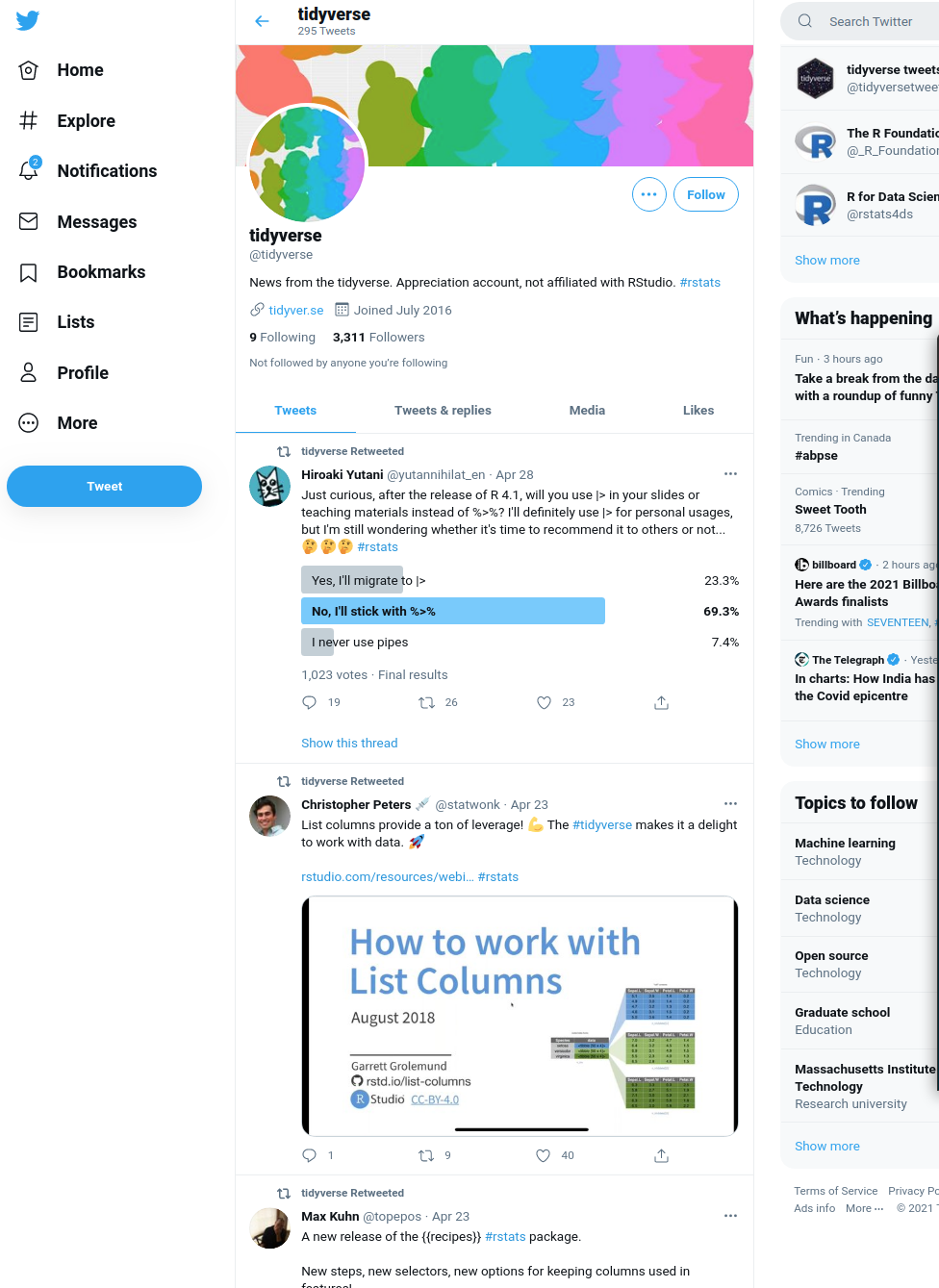
Fig. 10 The tidyverse account Twitter feed.
Stop! Think about your API usage carefully!
When you access an API, you are initiating a transfer of data from a web server to your computer. Web servers are expensive to run and do not have infinite resources. If you try to ask for too much data at once, you can use up a huge amount of the server’s bandwidth. If you try to ask for data too frequently—e.g., if you make many requests to the server in quick succession—you can also bog the server down and make it unable to talk to anyone else. Most servers have mechanisms to revoke your access if you are not careful, but you should try to prevent issues from happening in the first place by being extra careful with how you write and run your code. You should also keep in mind that when a website owner grants you API access, they also usually specify a limit (or quota) of how much data you can ask for. Be careful not to overrun your quota! In this example, we should take a look at the Twitter website to see what limits we should abide by when using the API.
Using rtweet
After checking the Twitter website, it seems like asking for 400 tweets one time is acceptable.
So we can use the get_timelines function to ask for the last 400 tweets from the @tidyverse account.
tidyverse_tweets <- get_timelines('tidyverse', n=400)
When you call the get_timelines for the first time (or any other rtweet function that accesses the API),
you will see a browser pop-up that looks something like Figure @ref(fig:01-tidyverse-authorize).
(ref:01-tidyverse-authorize) The rtweet authorization prompt.
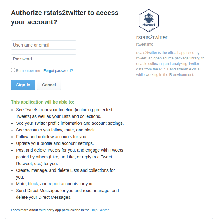
Fig. 11 (ref:01-tidyverse-authorize)
This is the rtweet package asking you to provide your own Twitter account’s login information.
When rtweet talks to the Twitter API, it uses your account information to authenticate requests;
Twitter then can keep track of how much data you’re asking for, and how frequently you’re asking.
If you want to follow along with this example using your own Twitter account, you should read
over the list of permissions you are granting rtweet very carefully and make sure you are comfortable
with it. Note that rtweet can be used to manage most aspects of your account (make posts, follow others, etc.),
which is why rtweet asks for such extensive permissions.
If you decide to allow rtweet to talk to the Twitter API using your account information, then
input your username and password and hit “Sign In.” Twitter will probably send you an email to say
that there was an unusual login attempt on your account, and in that case you will have to take
the one-time code they send you and provide that to the rtweet login page too.
Note: Every API has its own way to authenticate users when they try to access data. Many APIs require you to sign up to receive a token, which is a secret password that you input into the R package (like
rtweet) that you are using to access the API.
With the authentication setup out of the way, let’s run the get_timelines function again to actually access
the API and take a look at what was returned:
tidyverse_tweets <- get_timelines('tidyverse', n=400)
tidyverse_tweets
tidyverse_tweets <- read_csv("data/tweets.csv")
tidyverse_tweets
The data has quite a few variables! (Notice that the output above shows that we
have a data table with 293 rows and 71 columns). Let’s reduce this down to a
few variables of interest: created_at, retweet_screen_name, is_retweet,
and text.
tidyverse_tweets <- select(tidyverse_tweets,
                           created_at,
                           retweet_screen_name,
                           is_retweet,
                           text)

tidyverse_tweets
If you look back up at the image of the @tidyverse Twitter page, you will
recognize the text of the most recent few tweets in the above data frame. In
other words, we have successfully created a small data set using the Twitter
API—neat! This data is also quite different from what we obtained from web scraping;
it is already well-organized into a tidyverse data frame (although not every API
will provide data in such a nice format).
From this point onward, the tidyverse_tweets data frame is stored on your
machine, and you can play with it to your heart’s content. For example, you can use
write_csv to save it to a file and read_csv to read it into R again later;
and after reading the next few chapters you will have the skills to
compute the percentage of retweets versus tweets, find the most oft-retweeted
account, make visualizations of the data, and much more! If you decide that you want
to ask the Twitter API for more data
(see the rtweet page
for more examples of what is possible), just be mindful as usual about how much
data you are requesting and how frequently you are making requests.
Exercises
Practice exercises for the material covered in this chapter can be found in the accompanying worksheets repository in the “Reading in data locally and from the web” row. You can launch an interactive version of the worksheet in your browser by clicking the “launch binder” button. You can also preview a non-interactive version of the worksheet by clicking “view worksheet.” If you instead decide to download the worksheet and run it on your own machine, make sure to follow the instructions for computer setup found in Chapter @ref(move-to-your-own-machine). This will ensure that the automated feedback and guidance that the worksheets provide will function as intended.
Additional resources
The
readrdocumentation provides the documentation for many of the reading functions we cover in this chapter. It is where you should look if you want to learn more about the functions in this chapter, the full set of arguments you can use, and other related functions. The site also provides a very nice cheat sheet that summarizes many of the data wrangling functions from this chapter.Sometimes you might run into data in such poor shape that none of the reading functions we cover in this chapter work. In that case, you can consult the data import chapter from R for Data Science [@wickham2016r], which goes into a lot more detail about how R parses text from files into data frames.
The
hereR package [@here] provides a way for you to construct or find your files’ paths.The
readxldocumentation provides more details on reading data from Excel, such as reading in data with multiple sheets, or specifying the cells to read in.The
rioR package [@rio] provides an alternative set of tools for reading and writing data in R. It aims to be a “Swiss army knife” for data reading/writing/converting, and supports a wide variety of data types (including data formats generated by other statistical software like SPSS and SAS).A video from the Udacity course Linux Command Line Basics provides a good explanation of absolute versus relative paths.
If you read the subsection on obtaining data from the web via scraping and APIs, we provide two companion tutorial video links for how to use the SelectorGadget tool to obtain desired CSS selectors for:
The
politeR package [@polite] provides a set of tools for responsibly scraping data from websites.