Classification II: evaluation & tuning
Contents
Classification II: evaluation & tuning
Overview
This chapter continues the introduction to predictive modeling through classification. While the previous chapter covered training and data preprocessing, this chapter focuses on how to evaluate the accuracy of a classifier, as well as how to improve the classifier (where possible) to maximize its accuracy.
Chapter learning objectives
By the end of the chapter, readers will be able to do the following:
Describe what training, validation, and test data sets are and how they are used in classification.
Split data into training, validation, and test data sets.
Describe what a random seed is and its importance in reproducible data analysis.
Set the random seed in Python using the
numpy.random.seedfunction orrandom_stateargument in some of thescikit-learnfunctions.Evaluate classification accuracy in Python using a validation data set and appropriate metrics.
Execute cross-validation in Python to choose the number of neighbors in a \(K\)-nearest neighbors classifier.
Describe the advantages and disadvantages of the \(K\)-nearest neighbors classification algorithm.
Evaluating accuracy
Sometimes our classifier might make the wrong prediction. A classifier does not need to be right 100% of the time to be useful, though we don’t want the classifier to make too many wrong predictions. How do we measure how “good” our classifier is? Let’s revisit the \index{breast cancer} breast cancer images data [Street et al., 1993] and think about how our classifier will be used in practice. A biopsy will be performed on a new patient’s tumor, the resulting image will be analyzed, and the classifier will be asked to decide whether the tumor is benign or malignant. The key word here is new: our classifier is “good” if it provides accurate predictions on data not seen during training. But then, how can we evaluate our classifier without visiting the hospital to collect more tumor images?
The trick is to split the data into a training set \index{training set} and test set \index{test set} (Fig. 27) and use only the training set when building the classifier. Then, to evaluate the accuracy of the classifier, we first set aside the true labels from the test set, and then use the classifier to predict the labels in the test set. If our predictions match the true labels for the observations in the test set, then we have some confidence that our classifier might also accurately predict the class labels for new observations without known class labels.
Note: If there were a golden rule of machine learning, \index{golden rule of machine learning} it might be this: you cannot use the test data to build the model! If you do, the model gets to “see” the test data in advance, making it look more accurate than it really is. Imagine how bad it would be to overestimate your classifier’s accuracy when predicting whether a patient’s tumor is malignant or benign!
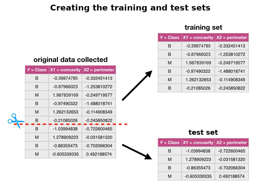
Fig. 27 Splitting the data into training and testing sets.
How exactly can we assess how well our predictions match the true labels for the observations in the test set? One way we can do this is to calculate the prediction accuracy. \index{prediction accuracy|see{accuracy}}\index{accuracy} This is the fraction of examples for which the classifier made the correct prediction. To calculate this, we divide the number of correct predictions by the number of predictions made.
The process for assessing if our predictions match the true labels in the test set is illustrated in Fig. 28. Note that there are other measures for how well classifiers perform, such as precision and recall; these will not be discussed here, but you will likely encounter them in other more advanced books on this topic.
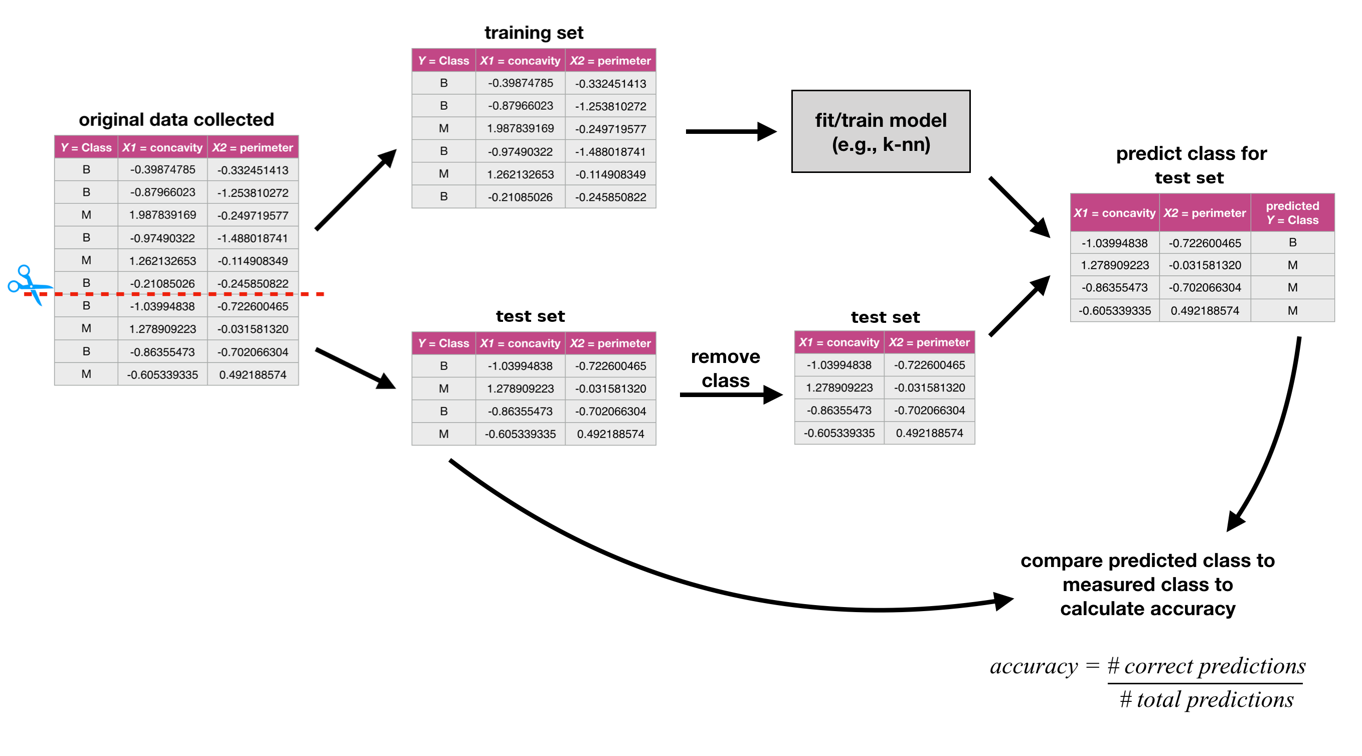
Fig. 28 Process for splitting the data and finding the prediction accuracy.
Randomness and seeds
Beginning in this chapter, our data analyses will often involve the use of randomness. \index{random} We use randomness any time we need to make a decision in our analysis that needs to be fair, unbiased, and not influenced by human input. For example, in this chapter, we need to split a data set into a training set and test set to evaluate our classifier. We certainly do not want to choose how to split the data ourselves by hand, as we want to avoid accidentally influencing the result of the evaluation. So instead, we let Python randomly split the data. In future chapters we will use randomness in many other ways, e.g., to help us select a small subset of data from a larger data set, to pick groupings of data, and more.
However, the use of randomness runs counter to one of the main
tenets of good data analysis practice: \index{reproducible} reproducibility. Recall that a reproducible
analysis produces the same result each time it is run; if we include randomness
in the analysis, would we not get a different result each time?
The trick is that in Python—and other programming languages—randomness
is not actually random! Instead, Python uses a random number generator that
produces a sequence of numbers that
are completely determined by a \index{seed} \index{random seed|see{seed}}
seed value. Once you set the seed value
using the \index{seed!set.seed} np.random.seed function or the random_state argument, everything after that point may look random,
but is actually totally reproducible. As long as you pick the same seed
value, you get the same result!
Let’s use an example to investigate how seeds work in Python. Say we want
to randomly pick 10 numbers from 0 to 9 in Python using the np.random.choice \index{sample!function} function,
but we want it to be reproducible. Before using the sample function,
we call np.random.seed, and pass it any integer as an argument.
Here, we pass in the number 1.
import numpy as np

np.random.seed(1)
random_numbers = np.random.choice(range(10), size=10, replace=True)
random_numbers
array([5, 8, 9, 5, 0, 0, 1, 7, 6, 9])
You can see that random_numbers is a list of 10 numbers
from 0 to 9 that, from all appearances, looks random. If
we run the np.random.choice function again, we will
get a fresh batch of 10 numbers that also look random.
random_numbers = np.random.choice(range(10), size=10, replace=True)
random_numbers
array([2, 4, 5, 2, 4, 2, 4, 7, 7, 9])
If we want to force Python to produce the same sequences of random numbers,
we can simply call the np.random.seed function again with the same argument
value.
np.random.seed(1)
random_numbers = np.random.choice(range(10), size=10, replace=True)
random_numbers
array([5, 8, 9, 5, 0, 0, 1, 7, 6, 9])
random_numbers = np.random.choice(range(10), size=10, replace=True)
random_numbers
array([2, 4, 5, 2, 4, 2, 4, 7, 7, 9])
And if we choose a different value for the seed—say, 4235—we obtain a different sequence of random numbers.
np.random.seed(4235)
random_numbers = np.random.choice(range(10), size=10, replace=True)
random_numbers
array([8, 0, 1, 0, 0, 7, 5, 5, 3, 9])
random_numbers = np.random.choice(range(10), size=10, replace=True)
random_numbers
array([7, 5, 9, 5, 5, 8, 2, 8, 0, 4])
In other words, even though the sequences of numbers that Python is generating look random, they are totally determined when we set a seed value!
So what does this mean for data analysis? Well, np.random.choice is certainly
not the only function that uses randomness in R. Many of the functions
that we use in scikit-learn, numpy, and beyond use randomness—many of them
without even telling you about it.
Also note that when Python starts up, it creates its own seed to use. So if you do not
explicitly call the np.random.seed function in your code or specify the random_state
argument in scikit-learn functions (where it is available), your results will
likely not be reproducible.
And finally, be careful to set the seed only once at the beginning of a data
analysis. Each time you set the seed, you are inserting your own human input,
thereby influencing the analysis. If you use np.random.choice many times
throughout your analysis, the randomness that Python uses will not look
as random as it should.
Different argument values in np.random.seed lead to different patterns of randomness, but as long as
you pick the same argument value your result will be the same.
Evaluating accuracy with scikit-learn
Back to evaluating classifiers now!
In Python, we can use the scikit-learn package \index{tidymodels} not only to perform \(K\)-nearest neighbors
classification, but also to assess how well our classification worked.
Let’s work through an example of how to use tools from scikit-learn to evaluate a classifier
using the breast cancer data set from the previous chapter.
We begin the analysis by loading the packages we require,
reading in the breast cancer data,
and then making a quick scatter plot visualization \index{visualization!scatter} of
tumor cell concavity versus smoothness colored by diagnosis in Fig. 29.
You will also notice that we set the random seed using either the np.random.seed function
or random_state argument, as described in Section Randomness and seeds.
# load packages
import altair as alt
import pandas as pd

# set the seed
np.random.seed(1)

# load data
cancer = pd.read_csv("data/unscaled_wdbc.csv")
## re-label Class 'M' as 'Malignant', and Class 'B' as 'Benign'
cancer["Class"] = cancer["Class"].apply(
    lambda x: "Malignant" if (x == "M") else "Benign"
)

# create scatter plot of tumor cell concavity versus smoothness,
# labeling the points be diagnosis class
## create a list of colors that will be used to customize the color of points
colors = ["#86bfef", "#efb13f"]

perim_concav = (
    alt.Chart(cancer)
    .mark_point(opacity=0.6, filled=True, size=40)
    .encode(
        x="Smoothness",
        y="Concavity",
        color=alt.Color("Class", scale=alt.Scale(range=colors), title="Diagnosis"),
    )
)

perim_concav

Fig. 29 Scatter plot of tumor cell concavity versus smoothness colored by diagnosis label.
Create the train / test split
Once we have decided on a predictive question to answer and done some preliminary exploration, the very next thing to do is to split the data into the training and test sets. Typically, the training set is between 50% and 95% of the data, while the test set is the remaining 5% to 50%; the intuition is that you want to trade off between training an accurate model (by using a larger training data set) and getting an accurate evaluation of its performance (by using a larger test data set). Here, we will use 75% of the data for training, and 25% for testing.
The train_test_split function \index{tidymodels!initial_split} from scikit-learn handles the procedure of splitting
the data for us. We can specify two very important parameters when using train_test_split to ensure
that the accuracy estimates from the test data are reasonable. First, shuffle=True (default) \index{shuffling} means the data will be shuffled before splitting, which ensures that any ordering present
in the data does not influence the data that ends up in the training and testing sets.
Second, by specifying the stratify parameter to be the target column of the training set,
it stratifies the \index{stratification} data by the class label, to ensure that roughly
the same proportion of each class ends up in both the training and testing sets. For example,
in our data set, roughly 63% of the
observations are from the benign class (Benign), and 37% are from the malignant class (Malignant),
so specifying stratify as the class column ensures that roughly 63% of the training data are benign,
37% of the training data are malignant,
and the same proportions exist in the testing data.
Let’s use the train_test_split function to create the training and testing sets.
We will specify that train_size=0.75 so that 75% of our original data set ends up
in the training set. We will also set the stratify argument to the categorical label variable
(here, cancer['Class']) to ensure that the training and testing subsets contain the
right proportions of each category of observation.
Note that the train_test_split function uses randomness, so we shall set random_state to make
the split reproducible.
cancer_train, cancer_test = train_test_split(
    cancer, train_size=0.75, stratify=cancer["Class"], random_state=1
)
cancer_train.info()
<class 'pandas.core.frame.DataFrame'>
Int64Index: 426 entries, 164 to 284
Data columns (total 12 columns):
 #   Column             Non-Null Count  Dtype
---  ------             --------------  -----
 0   ID                 426 non-null    int64
 1   Class              426 non-null    object
 2   Radius             426 non-null    float64
 3   Texture            426 non-null    float64
 4   Perimeter          426 non-null    float64
 5   Area               426 non-null    float64
 6   Smoothness         426 non-null    float64
 7   Compactness        426 non-null    float64
 8   Concavity          426 non-null    float64
 9   Concave_Points     426 non-null    float64
 10  Symmetry           426 non-null    float64
 11  Fractal_Dimension  426 non-null    float64
dtypes: float64(10), int64(1), object(1)
memory usage: 43.3+ KB
cancer_test.info()
<class 'pandas.core.frame.DataFrame'>
Int64Index: 143 entries, 357 to 332
Data columns (total 12 columns):
 #   Column             Non-Null Count  Dtype
---  ------             --------------  -----
 0   ID                 143 non-null    int64
 1   Class              143 non-null    object
 2   Radius             143 non-null    float64
 3   Texture            143 non-null    float64
 4   Perimeter          143 non-null    float64
 5   Area               143 non-null    float64
 6   Smoothness         143 non-null    float64
 7   Compactness        143 non-null    float64
 8   Concavity          143 non-null    float64
 9   Concave_Points     143 non-null    float64
 10  Symmetry           143 non-null    float64
 11  Fractal_Dimension  143 non-null    float64
dtypes: float64(10), int64(1), object(1)
memory usage: 14.5+ KB
We can see from .info() in \index{glimpse} the code above that the training set contains 426 observations,
while the test set contains 143 observations. This corresponds to
a train / test split of 75% / 25%, as desired. Recall from Chapter Classification I: training & predicting
that we use the .info() method to view data with a large number of columns,
as it prints the data such that the columns go down the page (instead of across).
We can use .groupby() and .count() to \index{group_by}\index{summarize} find the percentage of malignant and benign classes
in cancer_train and we see about 63% of the training
data are benign and 37%
are malignant, indicating that our class proportions were roughly preserved when we split the data.
cancer_proportions = pd.DataFrame()
cancer_proportions['n'] = cancer_train.groupby('Class')['ID'].count()
cancer_proportions['percent'] = 100 * cancer_proportions['n'] / len(cancer_train)
cancer_proportions
| n | percent | |
|---|---|---|
| Class | ||
| Benign | 267 | 62.676056 |
| Malignant | 159 | 37.323944 |
Preprocess the data
As we mentioned in the last chapter, \(K\)-nearest neighbors is sensitive to the scale of the predictors, so we should perform some preprocessing to standardize them. An additional consideration we need to take when doing this is that we should create the standardization preprocessor using only the training data. This ensures that our test data does not influence any aspect of our model training. Once we have created the standardization preprocessor, we can then apply it separately to both the training and test data sets.
Fortunately, the Pipeline framework (together with column transformer) from scikit-learn helps us handle this properly. Below we construct and prepare the preprocessor using make_column_transformer. Later after we construct a full Pipeline, we will only fit it with the training data.
cancer_preprocessor = make_column_transformer(
    (StandardScaler(), ["Smoothness", "Concavity"]),
)
Train the classifier
Now that we have split our original data set into training and test sets, we
can create our \(K\)-nearest neighbors classifier with only the training set using
the technique we learned in the previous chapter. For now, we will just choose
the number \(K\) of neighbors to be 3. To fit the model with only concavity and smoothness as the
predictors, we need to explicitly create X (predictors) and y (target) based on cancer_train.
As before we need to create a model specification, combine
the model specification and preprocessor into a workflow, and then finally
use fit with X and y to build the classifier.
# hidden seed
# np.random.seed(1)

knn_spec = KNeighborsClassifier(n_neighbors=3)  ## weights="uniform"

X = cancer_train.loc[:, ["Smoothness", "Concavity"]]
y = cancer_train["Class"]

knn_fit = make_pipeline(cancer_preprocessor, knn_spec).fit(X, y)

knn_fit
Pipeline(steps=[('columntransformer',
                 ColumnTransformer(transformers=[('standardscaler',
                                                  StandardScaler(),
                                                  ['Smoothness',
                                                   'Concavity'])])),
                ('kneighborsclassifier', KNeighborsClassifier(n_neighbors=3))])
In a Jupyter environment, please rerun this cell to show the HTML representation or trust the notebook. On GitHub, the HTML representation is unable to render, please try loading this page with nbviewer.org.
Pipeline(steps=[('columntransformer',
                 ColumnTransformer(transformers=[('standardscaler',
                                                  StandardScaler(),
                                                  ['Smoothness',
                                                   'Concavity'])])),
('kneighborsclassifier', KNeighborsClassifier(n_neighbors=3))])ColumnTransformer(transformers=[('standardscaler', StandardScaler(),
['Smoothness', 'Concavity'])])['Smoothness', 'Concavity']
StandardScaler()
KNeighborsClassifier(n_neighbors=3)
Predict the labels in the test set
Now that we have a \(K\)-nearest neighbors classifier object, we can use it to
predict the class labels for our test set. We use the pandas.concat() to add the
column of predictions to the original test data, creating the
cancer_test_predictions data frame. The Class variable contains the true
diagnoses, while the predicted contains the predicted diagnoses from the
classifier.
cancer_test_predictions = knn_fit.predict(
    cancer_test.loc[:, ["Smoothness", "Concavity"]]
)

cancer_test_predictions = pd.concat(
    [
        pd.DataFrame(cancer_test_predictions, columns=["predicted"]),
        cancer_test.reset_index(drop=True),
    ],
    axis=1,
)  # add the predictions column to the original test data

cancer_test_predictions
| predicted | ID | Class | Radius | Texture | Perimeter | Area | Smoothness | Compactness | Concavity | Concave_Points | Symmetry | Fractal_Dimension | |
|---|---|---|---|---|---|---|---|---|---|---|---|---|---|
| 0 | Benign | 901028 | Benign | 13.870 | 16.21 | 88.52 | 593.7 | 0.08743 | 0.05492 | 0.015020 | 0.020880 | 0.1424 | 0.05883 |
| 1 | Benign | 901041 | Benign | 13.300 | 21.57 | 85.24 | 546.1 | 0.08582 | 0.06373 | 0.033440 | 0.024240 | 0.1815 | 0.05696 |
| 2 | Malignant | 8810703 | Malignant | 28.110 | 18.47 | 188.50 | 2499.0 | 0.11420 | 0.15160 | 0.320100 | 0.159500 | 0.1648 | 0.05525 |
| 3 | Benign | 91813702 | Benign | 12.340 | 12.27 | 78.94 | 468.5 | 0.09003 | 0.06307 | 0.029580 | 0.026470 | 0.1689 | 0.05808 |
| 4 | Benign | 8510824 | Benign | 9.504 | 12.44 | 60.34 | 273.9 | 0.10240 | 0.06492 | 0.029560 | 0.020760 | 0.1815 | 0.06905 |
| ... | ... | ... | ... | ... | ... | ... | ... | ... | ... | ... | ... | ... | ... |
| 138 | Benign | 9010877 | Benign | 13.400 | 16.95 | 85.48 | 552.4 | 0.07937 | 0.05696 | 0.021810 | 0.014730 | 0.1650 | 0.05701 |
| 139 | Benign | 908469 | Benign | 14.860 | 16.94 | 94.89 | 673.7 | 0.08924 | 0.07074 | 0.033460 | 0.028770 | 0.1573 | 0.05703 |
| 140 | Benign | 892399 | Benign | 10.510 | 23.09 | 66.85 | 334.2 | 0.10150 | 0.06797 | 0.024950 | 0.018750 | 0.1695 | 0.06556 |
| 141 | Benign | 913512 | Benign | 11.680 | 16.17 | 75.49 | 420.5 | 0.11280 | 0.09263 | 0.042790 | 0.031320 | 0.1853 | 0.06401 |
| 142 | Benign | 897132 | Benign | 11.220 | 19.86 | 71.94 | 387.3 | 0.10540 | 0.06779 | 0.005006 | 0.007583 | 0.1940 | 0.06028 |
143 rows × 13 columns
Compute the accuracy
Finally, we can assess our classifier’s accuracy. To do this we use the score method
from scikit-learn to get the statistics about the quality of our model, specifying
the X and y arguments based on cancer_test.
# np.random.seed(1)

X_test = cancer_test.loc[:, ["Smoothness", "Concavity"]]
y_test = cancer_test["Class"]

cancer_acc_1 = knn_fit.score(X_test, y_test)

cancer_acc_1
0.8741258741258742
The output shows that the estimated accuracy of the classifier on the test data
was 87%.
We can also look at the confusion matrix for the classifier as a numpy array using the confusion_matrix function:
# np.random.seed(1)

confusion = confusion_matrix(
    cancer_test_predictions["Class"],
    cancer_test_predictions["predicted"],
    labels=knn_fit.classes_,
)

confusion
array([[82,  8],
       [10, 43]])
It is hard for us to interpret the confusion matrix as shown above. We could use the ConfusionMatrixDisplay function of the scikit-learn package to plot the confusion matrix.
from sklearn.metrics import ConfusionMatrixDisplay

confusion_display = ConfusionMatrixDisplay(
    confusion_matrix=confusion, display_labels=knn_fit.classes_
)
confusion_display.plot();
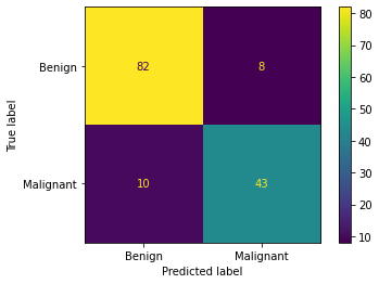
The confusion matrix shows 43 observations were correctly predicted
as malignant, and 82 were correctly predicted as benign. Therefore the classifier labeled
43 + 82 = 125 observations
correctly. It also shows that the classifier made some mistakes; in particular,
it classified 10 observations as benign when they were truly malignant,
and 8 observations as malignant when they were truly benign.
Critically analyze performance
We now know that the classifier was 87% accurate
on the test data set. That sounds pretty good! Wait, is it good?
Or do we need something higher?
In general, what a good value for accuracy \index{accuracy!assessment} is depends on the application. For instance, suppose you are predicting whether a tumor is benign or malignant for a type of tumor that is benign 99% of the time. It is very easy to obtain a 99% accuracy just by guessing benign for every observation. In this case, 99% accuracy is probably not good enough. And beyond just accuracy, sometimes the kind of mistake the classifier makes is important as well. In the previous example, it might be very bad for the classifier to predict “benign” when the true class is “malignant”, as this might result in a patient not receiving appropriate medical attention. On the other hand, it might be less bad for the classifier to guess “malignant” when the true class is “benign”, as the patient will then likely see a doctor who can provide an expert diagnosis. This is why it is important not only to look at accuracy, but also the confusion matrix.
However, there is always an easy baseline that you can compare to for any classification problem: the majority classifier. The majority classifier \index{classification!majority} always guesses the majority class label from the training data, regardless of the predictor variables’ values. It helps to give you a sense of scale when considering accuracies. If the majority classifier obtains a 90% accuracy on a problem, then you might hope for your \(K\)-nearest neighbors classifier to do better than that. If your classifier provides a significant improvement upon the majority classifier, this means that at least your method is extracting some useful information from your predictor variables. Be careful though: improving on the majority classifier does not necessarily mean the classifier is working well enough for your application.
As an example, in the breast cancer data, recall the proportions of benign and malignant observations in the training data are as follows:
cancer_proportions
| n | percent | |
|---|---|---|
| Class | ||
| Benign | 267 | 62.676056 |
| Malignant | 159 | 37.323944 |
Since the benign class represents the majority of the training data,
the majority classifier would always predict that a new observation
is benign. The estimated accuracy of the majority classifier is usually
fairly close to the majority class proportion in the training data.
In this case, we would suspect that the majority classifier will have
an accuracy of around 63%.
The \(K\)-nearest neighbors classifier we built does quite a bit better than this,
with an accuracy of 87%.
This means that from the perspective of accuracy,
the \(K\)-nearest neighbors classifier improved quite a bit on the basic
majority classifier. Hooray! But we still need to be cautious; in
this application, it is likely very important not to misdiagnose any malignant tumors to avoid missing
patients who actually need medical care. The confusion matrix above shows
that the classifier does, indeed, misdiagnose a significant number of malignant tumors as benign (10 out of 53 malignant tumors, or 19%!).
Therefore, even though the accuracy improved upon the majority classifier,
our critical analysis suggests that this classifier may not have appropriate performance
for the application.
Tuning the classifier
The vast majority of predictive models in statistics and machine learning have parameters. A parameter \index{parameter}\index{tuning parameter|see{parameter}} is a number you have to pick in advance that determines some aspect of how the model behaves. For example, in the \(K\)-nearest neighbors classification algorithm, \(K\) is a parameter that we have to pick that determines how many neighbors participate in the class vote. By picking different values of \(K\), we create different classifiers that make different predictions.
So then, how do we pick the best value of \(K\), i.e., tune the model? And is it possible to make this selection in a principled way? Ideally, we want somehow to maximize the performance of our classifier on data it hasn’t seen yet. But we cannot use our test data set in the process of building our model. So we will play the same trick we did before when evaluating our classifier: we’ll split our training data itself into two subsets, use one to train the model, and then use the other to evaluate it. In this section, we will cover the details of this procedure, as well as how to use it to help you pick a good parameter value for your classifier.
And remember: don’t touch the test set during the tuning process. Tuning is a part of model training!
Cross-validation
The first step in choosing the parameter \(K\) is to be able to evaluate the classifier using only the training data. If this is possible, then we can compare the classifier’s performance for different values of \(K\)—and pick the best—using only the training data. As suggested at the beginning of this section, we will accomplish this by splitting the training data, training on one subset, and evaluating on the other. The subset of training data used for evaluation is often called the validation set. \index{validation set}
There is, however, one key difference from the train/test split that we performed earlier. In particular, we were forced to make only a single split of the data. This is because at the end of the day, we have to produce a single classifier. If we had multiple different splits of the data into training and testing data, we would produce multiple different classifiers. But while we are tuning the classifier, we are free to create multiple classifiers based on multiple splits of the training data, evaluate them, and then choose a parameter value based on all of the different results. If we just split our overall training data once, our best parameter choice will depend strongly on whatever data was lucky enough to end up in the validation set. Perhaps using multiple different train/validation splits, we’ll get a better estimate of accuracy, which will lead to a better choice of the number of neighbors \(K\) for the overall set of training data.
Let’s investigate this idea in Python! In particular, we will generate five different train/validation splits of our overall training data, train five different \(K\)-nearest neighbors models, and evaluate their accuracy. We will start with just a single split.
# create the 25/75 split of the training data into training and validation
cancer_subtrain, cancer_validation = train_test_split(
    cancer_train, test_size=0.25, random_state=1
)

# could reuse the standardization preprocessor from before
# (but now we want to fit with the cancer_subtrain)
X = cancer_subtrain.loc[:, ["Smoothness", "Concavity"]]
y = cancer_subtrain["Class"]
knn_fit = make_pipeline(cancer_preprocessor, knn_spec).fit(X, y)

# get predictions on the validation data
validation_predicted = knn_fit.predict(
    cancer_validation.loc[:, ["Smoothness", "Concavity"]]
)
validation_predicted = pd.concat(
    [
        pd.DataFrame(validation_predicted, columns=["predicted"]),
        cancer_validation.reset_index(drop=True),
    ],
    axis=1,
)  # to add the predictions column to the original test data

# compute the accuracy
X_valid = cancer_validation.loc[:, ["Smoothness", "Concavity"]]
y_valid = cancer_validation["Class"]
acc = knn_fit.score(X_valid, y_valid)

acc
0.8691588785046729
The accuracy estimate using this split is 86.9%.
Now we repeat the above code 4 more times, which generates 4 more splits.
Therefore we get five different shuffles of the data, and therefore five different values for
accuracy: 86.9%, 85.0%, 87.9%,
86.9%, 87.9%. None of these values are
necessarily “more correct” than any other; they’re
just five estimates of the true, underlying accuracy of our classifier built
using our overall training data. We can combine the estimates by taking their
average (here 87%) to try to get a single assessment of our
classifier’s accuracy; this has the effect of reducing the influence of any one
(un)lucky validation set on the estimate.
In practice, we don’t use random splits, but rather use a more structured splitting procedure so that each observation in the data set is used in a validation set only a single time. The name for this strategy is cross-validation. In cross-validation, \index{cross-validation} we split our overall training data into \(C\) evenly sized chunks. Then, iteratively use \(1\) chunk as the validation set and combine the remaining \(C-1\) chunks as the training set. This procedure is shown in Fig. 30. Here, \(C=5\) different chunks of the data set are used, resulting in 5 different choices for the validation set; we call this 5-fold cross-validation.
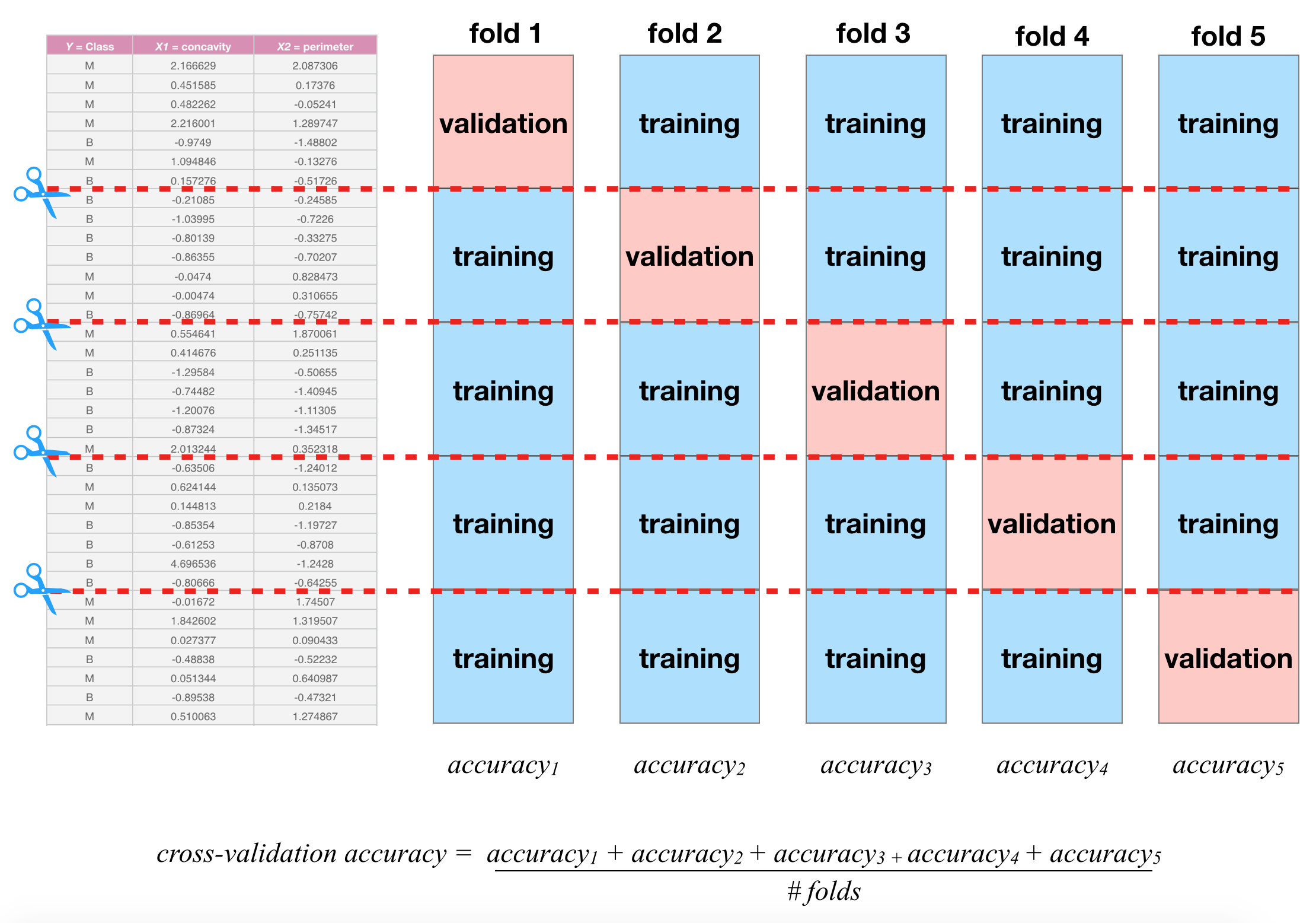
Fig. 30 5-fold cross-validation.
To perform 5-fold cross-validation in Python with scikit-learn, we use another
function: cross_validate. This function splits our training data into cv folds
automatically.
According to its documentation, the parameter cv:
For int/None inputs, if the estimator is a classifier and y is either binary or multiclass,
StratifiedKFoldis used.
This means cross_validate will ensure that the training and validation subsets contain the
right proportions of each category of observation.
When we run the cross_validate function, cross-validation is carried out on each
train/validation split. We can set return_train_score=True to obtain the training scores as well as the validation scores. The cross_validate function outputs a dictionary, and we use pd.DataFrame to convert it to a pandas dataframe for better visualization. (Noteworthy, the test_score column is actually the validation scores that we are interested in.)
cancer_pipe = make_pipeline(cancer_preprocessor, knn_spec)
X = cancer_subtrain.loc[:, ["Smoothness", "Concavity"]]
y = cancer_subtrain["Class"]
cv_5 = cross_validate(
    estimator=cancer_pipe,
    X=X,
    y=y,
    cv=5,
    return_train_score=True,
)

cv_5_df = pd.DataFrame(cv_5)
cv_5_df
| fit_time | score_time | test_score | train_score | |
|---|---|---|---|---|
| 0 | 0.005406 | 0.008005 | 0.828125 | 0.941176 |
| 1 | 0.004650 | 0.004558 | 0.890625 | 0.937255 |
| 2 | 0.004126 | 0.004287 | 0.890625 | 0.925490 |
| 3 | 0.004290 | 0.004182 | 0.890625 | 0.929412 |
| 4 | 0.004243 | 0.004412 | 0.873016 | 0.917969 |
We can then aggregate the mean and standard error
of the classifier’s validation accuracy across the folds.
You should consider the mean (mean) to be the estimated accuracy, while the standard
error (std) is a measure of how uncertain we are in the mean value. A detailed treatment of this
is beyond the scope of this chapter; but roughly, if your estimated mean is 0.87 and standard
error is 0.03, you can expect the true average accuracy of the
classifier to be somewhere roughly between 84% and 90% (although it may
fall outside this range). You may ignore the other columns in the metrics data frame.
cv_5_metrics = cv_5_df.aggregate(func=['mean', 'std'])
cv_5_metrics
| fit_time | score_time | test_score | train_score | |
|---|---|---|---|---|
| mean | 0.004543 | 0.005089 | 0.874603 | 0.930260 |
| std | 0.000521 | 0.001636 | 0.027078 | 0.009255 |
We can choose any number of folds, and typically the more we use the better our accuracy estimate will be (lower standard error). However, we are limited by computational power: the more folds we choose, the more computation it takes, and hence the more time it takes to run the analysis. So when you do cross-validation, you need to consider the size of the data, the speed of the algorithm (e.g., \(K\)-nearest neighbors), and the speed of your computer. In practice, this is a trial-and-error process, but typically \(C\) is chosen to be either 5 or 10. Here we will try 10-fold cross-validation to see if we get a lower standard error:
cv_10 = cross_validate(
    estimator=cancer_pipe,
    X=X,
    y=y,
    cv=10,
    return_train_score=True,
)

cv_10_df = pd.DataFrame(cv_10)
cv_10_metrics = cv_10_df.aggregate(func=['mean', 'std'])
cv_10_metrics
| fit_time | score_time | test_score | train_score | |
|---|---|---|---|---|
| mean | 0.004680 | 0.003783 | 0.877520 | 0.932428 |
| std | 0.000842 | 0.000481 | 0.065672 | 0.008401 |
In this case, using 10-fold instead of 5-fold cross validation did increase the standard error. In fact, due to the randomness in how the data are split, sometimes you might even end up with a lower standard error when increasing the number of folds! The increase in standard error can become more dramatic by increasing the number of folds by a large amount. In the following code we show the result when \(C = 50\); picking such a large number of folds often takes a long time to run in practice, so we usually stick to 5 or 10.
cv_50 = cross_validate(
    estimator=cancer_pipe,
    X=X,
    y=y,
    cv=50,
    return_train_score=True,
)

cv_50_df = pd.DataFrame(cv_50)
cv_50_metrics = cv_50_df.aggregate(func=['mean', 'std'])
cv_50_metrics
| fit_time | score_time | test_score | train_score | |
|---|---|---|---|---|
| mean | 0.004237 | 0.002794 | 0.879524 | 0.936345 |
| std | 0.000307 | 0.000329 | 0.129824 | 0.002509 |
Parameter value selection
Using 5- and 10-fold cross-validation, we have estimated that the prediction
accuracy of our classifier is somewhere around 88%.
Whether that is good or not
depends entirely on the downstream application of the data analysis. In the
present situation, we are trying to predict a tumor diagnosis, with expensive,
damaging chemo/radiation therapy or patient death as potential consequences of
misprediction. Hence, we might like to
do better than 88% for this application.
In order to improve our classifier, we have one choice of parameter: the number of
neighbors, \(K\). Since cross-validation helps us evaluate the accuracy of our
classifier, we can use cross-validation to calculate an accuracy for each value
of \(K\) in a reasonable range, and then pick the value of \(K\) that gives us the
best accuracy. The scikit-learn package collection provides 2 build-in methods for tuning parameters. Each parameter in the model can be adjusted rather than given a specific value. We can define a set of values for each hyperparameters and find the best parameters in this set.
Exhaustive grid search
A user specifies a set of values for each hyperparameter.
The method considers product of the sets and then evaluates each combination one by one.
Randomized hyperparameter optimization
Samples configurations at random until certain budget (e.g., time) is exhausted
Let us walk through how to use GridSearchCV to tune the model. RandomizedSearchCV follows a similar workflow, and you will get to practice both of them in the worksheet.
Before we use GridSearchCV (or RandomizedSearchCV), we should define the parameter grid by passing the set of values for each parameters that you would like to tune in a Python dictionary; below we create the param_grid dictionary with kneighborsclassifier__n_neighbors as the key and pair it with the values we would like to tune from 1 to 100 (stepping by 5) using the range function. We would also need to redefine the pipeline to use default values for parameters.
param_grid = {
    "kneighborsclassifier__n_neighbors": range(1, 100, 5),
}
cancer_tune_pipe = make_pipeline(cancer_preprocessor, KNeighborsClassifier())
Now, let us create the GridSearchCV object and the RandomizedSearchCV object by passing the new pipeline cancer_tune_pipe and the param_grid dictionary to the respective functions. n_jobs=-1 means using all the available processors.
cancer_tune_grid = GridSearchCV(
    estimator=cancer_tune_pipe,
    param_grid=param_grid,
    cv=10,
    n_jobs=-1,
    return_train_score=True,
)
Now, let us fit the model to the training data. The attribute cv_results_ of the fitted model is a dictionary of numpy arrays containing all cross-validation results from different choices of parameters. We can visualize them more clearly through a dataframe.
X_tune = cancer_train.loc[:, ["Smoothness", "Concavity"]]
y_tune = cancer_train["Class"]

cancer_model_grid = cancer_tune_grid.fit(X_tune, y_tune)

accuracies_grid = pd.DataFrame(cancer_model_grid.cv_results_)
accuracies_grid.info()
<class 'pandas.core.frame.DataFrame'>
RangeIndex: 20 entries, 0 to 19
Data columns (total 31 columns):
 #   Column                                   Non-Null Count  Dtype
---  ------                                   --------------  -----
 0   mean_fit_time                            20 non-null     float64
 1   std_fit_time                             20 non-null     float64
 2   mean_score_time                          20 non-null     float64
 3   std_score_time                           20 non-null     float64
 4   param_kneighborsclassifier__n_neighbors  20 non-null     object
 5   params                                   20 non-null     object
 6   split0_test_score                        20 non-null     float64
 7   split1_test_score                        20 non-null     float64
 8   split2_test_score                        20 non-null     float64
 9   split3_test_score                        20 non-null     float64
 10  split4_test_score                        20 non-null     float64
 11  split5_test_score                        20 non-null     float64
 12  split6_test_score                        20 non-null     float64
 13  split7_test_score                        20 non-null     float64
 14  split8_test_score                        20 non-null     float64
 15  split9_test_score                        20 non-null     float64
 16  mean_test_score                          20 non-null     float64
 17  std_test_score                           20 non-null     float64
 18  rank_test_score                          20 non-null     int32
 19  split0_train_score                       20 non-null     float64
 20  split1_train_score                       20 non-null     float64
 21  split2_train_score                       20 non-null     float64
 22  split3_train_score                       20 non-null     float64
 23  split4_train_score                       20 non-null     float64
 24  split5_train_score                       20 non-null     float64
 25  split6_train_score                       20 non-null     float64
 26  split7_train_score                       20 non-null     float64
 27  split8_train_score                       20 non-null     float64
 28  split9_train_score                       20 non-null     float64
 29  mean_train_score                         20 non-null     float64
 30  std_train_score                          20 non-null     float64
dtypes: float64(28), int32(1), object(2)
memory usage: 4.9+ KB
cv_results_ gives abundant information, but for our purpose, we only focus on param_kneighborsclassifier__n_neighbors (the \(K\), number of neighbors), mean_test_score (the mean validation score across all folds), and std_test_score (the standard deviation of the validation scores).
accuracies_grid[
    ["param_kneighborsclassifier__n_neighbors", "mean_test_score", "std_test_score"]
]
| param_kneighborsclassifier__n_neighbors | mean_test_score | std_test_score | |
|---|---|---|---|
| 0 | 1 | 0.852436 | 0.051659 |
| 1 | 6 | 0.885271 | 0.059977 |
| 2 | 11 | 0.875914 | 0.047283 |
| 3 | 16 | 0.882946 | 0.048476 |
| 4 | 21 | 0.889978 | 0.045175 |
| 5 | 26 | 0.887597 | 0.039597 |
| 6 | 31 | 0.887597 | 0.039597 |
| 7 | 36 | 0.887542 | 0.035418 |
| 8 | 41 | 0.887542 | 0.035418 |
| 9 | 46 | 0.889922 | 0.035694 |
| 10 | 51 | 0.889867 | 0.037330 |
| 11 | 56 | 0.887431 | 0.040142 |
| 12 | 61 | 0.878128 | 0.041255 |
| 13 | 66 | 0.871041 | 0.037627 |
| 14 | 71 | 0.873367 | 0.039031 |
| 15 | 76 | 0.878073 | 0.043793 |
| 16 | 81 | 0.880399 | 0.044641 |
| 17 | 86 | 0.875748 | 0.041520 |
| 18 | 91 | 0.878018 | 0.046417 |
| 19 | 96 | 0.871041 | 0.044410 |
We can decide which number of neighbors is best by plotting the accuracy versus \(K\), as shown in Fig. 31.
accuracy_vs_k = (
    alt.Chart(accuracies_grid)
    .mark_line(point=True)
    .encode(
        x=alt.X(
            "param_kneighborsclassifier__n_neighbors",
            title="Neighbors",
        ),
        y=alt.Y(
            "mean_test_score",
            title="Accuracy estimate",
            scale=alt.Scale(domain=(0.85, 0.90)),
        ),
    )
)

accuracy_vs_k
Fig. 31 Plot of estimated accuracy versus the number of neighbors.
Setting the number of
neighbors to \(K =\) 21
provides the highest accuracy (89.0%). But there is no exact or perfect answer here;
any selection from \(K = 20\) and \(55\) would be reasonably justified, as all
of these differ in classifier accuracy by a small amount. Remember: the
values you see on this plot are estimates of the true accuracy of our
classifier. Although the
\(K =\) 21 value is
higher than the others on this plot,
that doesn’t mean the classifier is actually more accurate with this parameter
value! Generally, when selecting \(K\) (and other parameters for other predictive
models), we are looking for a value where:
we get roughly optimal accuracy, so that our model will likely be accurate;
changing the value to a nearby one (e.g., adding or subtracting a small number) doesn’t decrease accuracy too much, so that our choice is reliable in the presence of uncertainty;
the cost of training the model is not prohibitive (e.g., in our situation, if \(K\) is too large, predicting becomes expensive!).
We know that \(K =\) 21
provides the highest estimated accuracy. Further, Fig. 31 shows that the estimated accuracy
changes by only a small amount if we increase or decrease \(K\) near \(K =\) 21.
And finally, \(K =\) 21 does not create a prohibitively expensive
computational cost of training. Considering these three points, we would indeed select
\(K =\) 21 for the classifier.
Under/Overfitting
To build a bit more intuition, what happens if we keep increasing the number of
neighbors \(K\)? In fact, the accuracy actually starts to decrease!
Let’s specify a much larger range of values of \(K\) to try in the param_grid
argument of GridSearchCV. Fig. 32 shows a plot of estimated accuracy as
we vary \(K\) from 1 to almost the number of observations in the data set.
param_grid_lots = {
    "kneighborsclassifier__n_neighbors": range(1, 385, 10),
}

cancer_tune_grid_lots = GridSearchCV(
    estimator=cancer_tune_pipe,
    param_grid=param_grid_lots,
    cv=10,
    n_jobs=-1,
    return_train_score=True,
)

cancer_model_grid_lots = cancer_tune_grid_lots.fit(X_tune, y_tune)
accuracies_grid_lots = pd.DataFrame(cancer_model_grid_lots.cv_results_)

accuracy_vs_k_lots = (
    alt.Chart(accuracies_grid_lots)
    .mark_line(point=True)
    .encode(
        x=alt.X(
            "param_kneighborsclassifier__n_neighbors",
            title="Neighbors",
        ),
        y=alt.Y(
            "mean_test_score",
            title="Accuracy estimate",
            scale=alt.Scale(domain=(0.60, 0.90)),
        ),
    )
)

accuracy_vs_k_lots
Fig. 32 Plot of accuracy estimate versus number of neighbors for many K values.
Underfitting: \index{underfitting!classification} What is actually happening to our classifier that causes this? As we increase the number of neighbors, more and more of the training observations (and those that are farther and farther away from the point) get a “say” in what the class of a new observation is. This causes a sort of “averaging effect” to take place, making the boundary between where our classifier would predict a tumor to be malignant versus benign to smooth out and become simpler. If you take this to the extreme, setting \(K\) to the total training data set size, then the classifier will always predict the same label regardless of what the new observation looks like. In general, if the model isn’t influenced enough by the training data, it is said to underfit the data.
Overfitting: \index{overfitting!classification} In contrast, when we decrease the number of neighbors, each individual data point has a stronger and stronger vote regarding nearby points. Since the data themselves are noisy, this causes a more “jagged” boundary corresponding to a less simple model. If you take this case to the extreme, setting \(K = 1\), then the classifier is essentially just matching each new observation to its closest neighbor in the training data set. This is just as problematic as the large \(K\) case, because the classifier becomes unreliable on new data: if we had a different training set, the predictions would be completely different. In general, if the model is influenced too much by the training data, it is said to overfit the data.
Fig. 33 Effect of K in overfitting and underfitting.
Both overfitting and underfitting are problematic and will lead to a model that does not generalize well to new data. When fitting a model, we need to strike a balance between the two. You can see these two effects in Fig. 33, which shows how the classifier changes as we set the number of neighbors \(K\) to 1, 7, 20, and 300.
Summary
Classification algorithms use one or more quantitative variables to predict the value of another categorical variable. In particular, the \(K\)-nearest neighbors algorithm does this by first finding the \(K\) points in the training data nearest to the new observation, and then returning the majority class vote from those training observations. We can evaluate a classifier by splitting the data randomly into a training and test data set, using the training set to build the classifier, and using the test set to estimate its accuracy. Finally, we can tune the classifier (e.g., select the number of neighbors \(K\) in \(K\)-NN) by maximizing estimated accuracy via cross-validation. The overall process is summarized in Fig. 34.
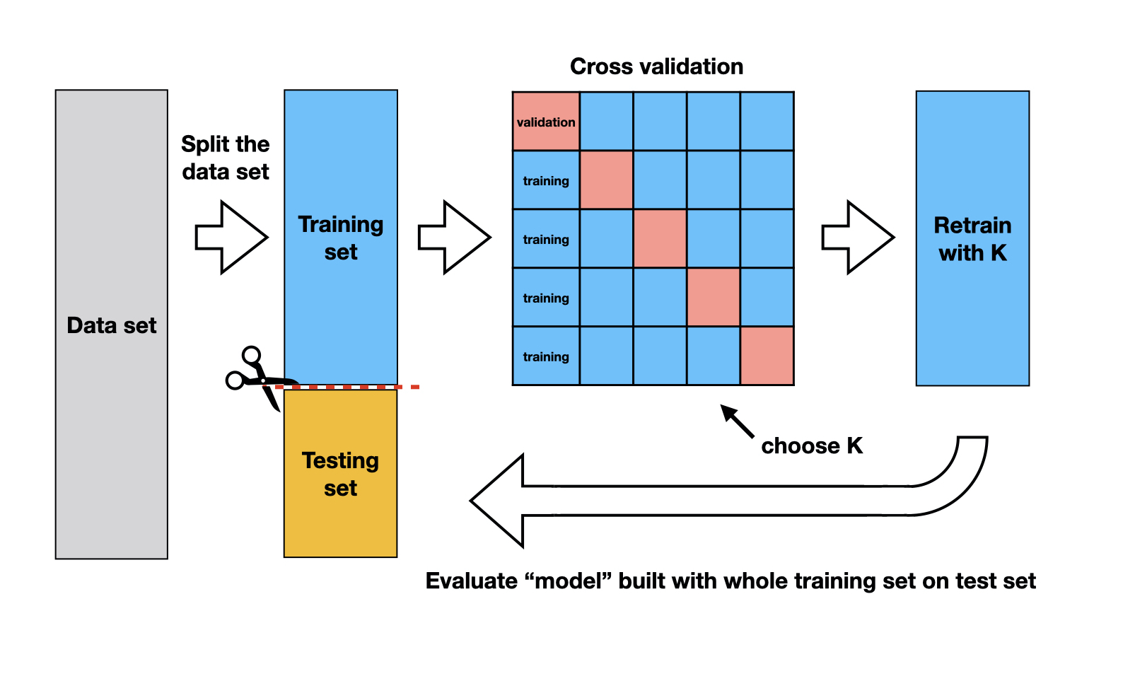
Fig. 34 Overview of KNN classification.
The overall workflow for performing \(K\)-nearest neighbors classification using scikit-learn is as follows:
Use the
train_test_splitfunction to split the data into a training and test set. Set thestratifyargument to the class label column of the dataframe. Put the test set aside for now.Define the parameter grid by passing the set of \(K\) values that you would like to tune.
Create a
Pipelinethat specifies the preprocessing steps and the classifier.Use the
GridSearchCVfunction (orRandomizedSearchCV) to estimate the classifier accuracy for a range of \(K\) values. Pass the parameter grid and the pipeline defined in step 2 and step 3 as theparam_gridargument and theestimatorargument, respectively.Call
fiton theGridSearchCVinstance created in step 4, passing the training data.Pick a value of \(K\) that yields a high accuracy estimate that doesn’t change much if you change \(K\) to a nearby value.
Make a new model specification for the best parameter value (i.e., \(K\)), and retrain the classifier by calling the
fitmethod.Evaluate the estimated accuracy of the classifier on the test set using the
scoremethod.
In these last two chapters, we focused on the \(K\)-nearest neighbor algorithm, but there are many other methods we could have used to predict a categorical label. All algorithms have their strengths and weaknesses, and we summarize these for the \(K\)-NN here.
Strengths: \(K\)-nearest neighbors classification
is a simple, intuitive algorithm,
requires few assumptions about what the data must look like, and
works for binary (two-class) and multi-class (more than 2 classes) classification problems.
Weaknesses: \(K\)-nearest neighbors classification
becomes very slow as the training data gets larger,
may not perform well with a large number of predictors, and
may not perform well when classes are imbalanced.
Predictor variable selection
Note: This section is not required reading for the remainder of the textbook. It is included for those readers interested in learning how irrelevant variables can influence the performance of a classifier, and how to pick a subset of useful variables to include as predictors.
Another potentially important part of tuning your classifier is to choose which variables from your data will be treated as predictor variables. Technically, you can choose anything from using a single predictor variable to using every variable in your data; the \(K\)-nearest neighbors algorithm accepts any number of predictors. However, it is not the case that using more predictors always yields better predictions! In fact, sometimes including irrelevant predictors \index{irrelevant predictors} can actually negatively affect classifier performance.
The effect of irrelevant predictors
Let’s take a look at an example where \(K\)-nearest neighbors performs
worse when given more predictors to work with. In this example, we modified
the breast cancer data to have only the Smoothness, Concavity, and
Perimeter variables from the original data. Then, we added irrelevant
variables that we created ourselves using a random number generator.
The irrelevant variables each take a value of 0 or 1 with equal probability for each observation, regardless
of what the value Class variable takes. In other words, the irrelevant variables have
no meaningful relationship with the Class variable.
cancer_irrelevant[
    ["Class", "Smoothness", "Concavity", "Perimeter", "Irrelevant1", "Irrelevant2"]
]
| Class | Smoothness | Concavity | Perimeter | Irrelevant1 | Irrelevant2 | |
|---|---|---|---|---|---|---|
| 0 | Malignant | 0.11840 | 0.30010 | 122.80 | 0 | 1 |
| 1 | Malignant | 0.08474 | 0.08690 | 132.90 | 0 | 1 |
| 2 | Malignant | 0.10960 | 0.19740 | 130.00 | 1 | 0 |
| 3 | Malignant | 0.14250 | 0.24140 | 77.58 | 1 | 0 |
| 4 | Malignant | 0.10030 | 0.19800 | 135.10 | 1 | 0 |
| ... | ... | ... | ... | ... | ... | ... |
| 564 | Malignant | 0.11100 | 0.24390 | 142.00 | 0 | 0 |
| 565 | Malignant | 0.09780 | 0.14400 | 131.20 | 0 | 1 |
| 566 | Malignant | 0.08455 | 0.09251 | 108.30 | 1 | 1 |
| 567 | Malignant | 0.11780 | 0.35140 | 140.10 | 0 | 0 |
| 568 | Benign | 0.05263 | 0.00000 | 47.92 | 1 | 1 |
569 rows × 6 columns
Next, we build a sequence of \(K\)-NN classifiers that include Smoothness,
Concavity, and Perimeter as predictor variables, but also increasingly many irrelevant
variables. In particular, we create 6 data sets with 0, 5, 10, 15, 20, and 40 irrelevant predictors.
Then we build a model, tuned via 5-fold cross-validation, for each data set.
Fig. 35 shows
the estimated cross-validation accuracy versus the number of irrelevant predictors. As
we add more irrelevant predictor variables, the estimated accuracy of our
classifier decreases. This is because the irrelevant variables add a random
amount to the distance between each pair of observations; the more irrelevant
variables there are, the more (random) influence they have, and the more they
corrupt the set of nearest neighbors that vote on the class of the new
observation to predict.
Fig. 35 Effect of inclusion of irrelevant predictors.
Although the accuracy decreases as expected, one surprising thing about
Fig. 35 is that it shows that the method
still outperforms the baseline majority classifier (with about 63% accuracy)
even with 40 irrelevant variables.
How could that be? Fig. 36 provides the answer:
the tuning procedure for the \(K\)-nearest neighbors classifier combats the extra randomness from the irrelevant variables
by increasing the number of neighbors. Of course, because of all the extra noise in the data from the irrelevant
variables, the number of neighbors does not increase smoothly; but the general trend is increasing. Fig. 37 corroborates
this evidence; if we fix the number of neighbors to \(K=3\), the accuracy falls off more quickly.
Fig. 36 Tuned number of neighbors for varying number of irrelevant predictors.
Fig. 37 Accuracy versus number of irrelevant predictors for tuned and untuned number of neighbors.
Finding a good subset of predictors
So then, if it is not ideal to use all of our variables as predictors without consideration, how
do we choose which variables we should use? A simple method is to rely on your scientific understanding
of the data to tell you which variables are not likely to be useful predictors. For example, in the cancer
data that we have been studying, the ID variable is just a unique identifier for the observation.
As it is not related to any measured property of the cells, the ID variable should therefore not be used
as a predictor. That is, of course, a very clear-cut case. But the decision for the remaining variables
is less obvious, as all seem like reasonable candidates. It
is not clear which subset of them will create the best classifier. One could use visualizations and
other exploratory analyses to try to help understand which variables are potentially relevant, but
this process is both time-consuming and error-prone when there are many variables to consider.
Therefore we need a more systematic and programmatic way of choosing variables.
This is a very difficult problem to solve in
general, and there are a number of methods that have been developed that apply
in particular cases of interest. Here we will discuss two basic
selection methods as an introduction to the topic. See the additional resources at the end of
this chapter to find out where you can learn more about variable selection, including more advanced methods.
The first idea you might think of for a systematic way to select predictors is to try all possible subsets of predictors and then pick the set that results in the “best” classifier. This procedure is indeed a well-known variable selection method referred to as best subset selection [Beale et al., 1967, Hocking and Leslie, 1967]. \index{variable selection!best subset}\index{predictor selection|see{variable selection}} In particular, you
create a separate model for every possible subset of predictors,
tune each one using cross-validation, and
pick the subset of predictors that gives you the highest cross-validation accuracy.
Best subset selection is applicable to any classification method (\(K\)-NN or otherwise). However, it becomes very slow when you have even a moderate number of predictors to choose from (say, around 10). This is because the number of possible predictor subsets grows very quickly with the number of predictors, and you have to train the model (itself a slow process!) for each one. For example, if we have \(2\) predictors—let’s call them A and B—then we have 3 variable sets to try: A alone, B alone, and finally A and B together. If we have \(3\) predictors—A, B, and C—then we have 7 to try: A, B, C, AB, BC, AC, and ABC. In general, the number of models we have to train for \(m\) predictors is \(2^m-1\); in other words, when we get to \(10\) predictors we have over one thousand models to train, and at \(20\) predictors we have over one million models to train! So although it is a simple method, best subset selection is usually too computationally expensive to use in practice.
Another idea is to iteratively build up a model by adding one predictor variable at a time. This method—known as forward selection [Draper and Smith, 1966, Eforymson, 1966]—is also widely \index{variable selection!forward} applicable and fairly straightforward. It involves the following steps:
Start with a model having no predictors.
Run the following 3 steps until you run out of predictors:
For each unused predictor, add it to the model to form a candidate model.
Tune all of the candidate models.
Update the model to be the candidate model with the highest cross-validation accuracy.
Select the model that provides the best trade-off between accuracy and simplicity.
Say you have \(m\) total predictors to work with. In the first iteration, you have to make \(m\) candidate models, each with 1 predictor. Then in the second iteration, you have to make \(m-1\) candidate models, each with 2 predictors (the one you chose before and a new one). This pattern continues for as many iterations as you want. If you run the method all the way until you run out of predictors to choose, you will end up training \(\frac{1}{2}m(m+1)\) separate models. This is a big improvement from the \(2^m-1\) models that best subset selection requires you to train! For example, while best subset selection requires training over 1000 candidate models with \(m=10\) predictors, forward selection requires training only 55 candidate models. Therefore we will continue the rest of this section using forward selection.
Note: One word of caution before we move on. Every additional model that you train increases the likelihood that you will get unlucky and stumble on a model that has a high cross-validation accuracy estimate, but a low true accuracy on the test data and other future observations. Since forward selection involves training a lot of models, you run a fairly high risk of this happening. To keep this risk low, only use forward selection when you have a large amount of data and a relatively small total number of predictors. More advanced methods do not suffer from this problem as much; see the additional resources at the end of this chapter for where to learn more about advanced predictor selection methods.
Forward selection in Python
We now turn to implementing forward selection in Python.
The function SequentialFeatureSelector
in the scikit-learn can automate this for us, and a simple demo is shown below. However, for
the learning purpose, we also want to show how each predictor is selected over iterations,
so we will have to code it ourselves.
First we will extract the “total” set of predictors that we are willing to work with.
Here we will load the modified version of the cancer data with irrelevant
predictors, and select Smoothness, Concavity, Perimeter, Irrelevant1, Irrelevant2, and Irrelevant3
as potential predictors, and the Class variable as the label.
We will also extract the column names for the full set of predictor variables.
cancer_subset = cancer_irrelevant[
    [
        "Class",
        "Smoothness",
        "Concavity",
        "Perimeter",
        "Irrelevant1",
        "Irrelevant2",
        "Irrelevant3",
    ]
]

names = list(cancer_subset.drop(
    columns=["Class"]
).columns.values)

cancer_subset
| Class | Smoothness | Concavity | Perimeter | Irrelevant1 | Irrelevant2 | Irrelevant3 | |
|---|---|---|---|---|---|---|---|
| 0 | Malignant | 0.11840 | 0.30010 | 122.80 | 0 | 1 | 0 |
| 1 | Malignant | 0.08474 | 0.08690 | 132.90 | 0 | 1 | 0 |
| 2 | Malignant | 0.10960 | 0.19740 | 130.00 | 1 | 0 | 0 |
| 3 | Malignant | 0.14250 | 0.24140 | 77.58 | 1 | 0 | 0 |
| 4 | Malignant | 0.10030 | 0.19800 | 135.10 | 1 | 0 | 1 |
| ... | ... | ... | ... | ... | ... | ... | ... |
| 564 | Malignant | 0.11100 | 0.24390 | 142.00 | 0 | 0 | 0 |
| 565 | Malignant | 0.09780 | 0.14400 | 131.20 | 0 | 1 | 0 |
| 566 | Malignant | 0.08455 | 0.09251 | 108.30 | 1 | 1 | 0 |
| 567 | Malignant | 0.11780 | 0.35140 | 140.10 | 0 | 0 | 0 |
| 568 | Benign | 0.05263 | 0.00000 | 47.92 | 1 | 1 | 1 |
569 rows × 7 columns
# Using scikit-learn SequentialFeatureSelector
from sklearn.feature_selection import SequentialFeatureSelector
cancer_preprocessor = make_column_transformer(
    (
        StandardScaler(),
        list(cancer_subset.drop(columns=["Class"]).columns),
    ),
)

cancer_pipe_forward = make_pipeline(
    cancer_preprocessor,
    SequentialFeatureSelector(KNeighborsClassifier(), direction="forward"),
    KNeighborsClassifier(),
)

X = cancer_subset.drop(columns=["Class"])
y = cancer_subset["Class"]

cancer_pipe_forward.fit(X, y)

cancer_pipe_forward.named_steps['sequentialfeatureselector'].n_features_to_select_
/opt/miniconda3/envs/dsci100/lib/python3.9/site-packages/sklearn/feature_selection/_sequential.py:188: FutureWarning: Leaving `n_features_to_select` to None is deprecated in 1.0 and will become 'auto' in 1.3. To keep the same behaviour as with None (i.e. select half of the features) and avoid this warning, you should manually set `n_features_to_select='auto'` and set tol=None when creating an instance.
  warnings.warn(
3
This means that 3 features were selected according to the forward selection algorithm.
Now, let’s code the actual algorithm by ourselves. The key idea of the forward selection code is to properly extract each subset of predictors for which we want to build a model, pass them to the preprocessor and fit the pipeline with them.
Finally, we need to write some code that performs the task of sequentially
finding the best predictor to add to the model.
If you recall the end of the wrangling chapter, we mentioned
that sometimes one needs more flexible forms of iteration than what
we have used earlier, and in these cases one typically resorts to
a for loop; see the section on control flow (for loops) in Python for Data Analysis [McKinney, 2012].
Here we will use two for loops:
one over increasing predictor set sizes
(where you see for i in range(1, n_total + 1): below),
and another to check which predictor to add in each round (where you see for j in range(len(names)) below).
For each set of predictors to try, we extract the subset of predictors,
pass it into a preprocessor, build a Pipeline that tunes
a \(K\)-NN classifier using 10-fold cross-validation,
and finally records the estimated accuracy.
accuracy_dict = {"size": [], "selected_predictors": [], "accuracy": []}

# store the total number of predictors
n_total = len(names)

selected = []

# for every possible number of predictors
for i in range(1, n_total + 1):
    accs = []
    models = []
    for j in range(len(names)):
        # create the preprocessor and pipeline with specified set of predictors
        cancer_preprocessor = make_column_transformer(
            (StandardScaler(), selected + [names[j]]),
        )
        cancer_tune_pipe = make_pipeline(cancer_preprocessor, KNeighborsClassifier())
        # tune the KNN classifier with these predictors,
        # and collect the accuracy for the best K
        param_grid = {
            "kneighborsclassifier__n_neighbors": range(1, 61, 5),
        }  ## double check

        cancer_tune_grid = GridSearchCV(
            estimator=cancer_tune_pipe,
            param_grid=param_grid,
            cv=10,  ## double check
            n_jobs=-1,
            # return_train_score=True,
        )

        X = cancer_subset[selected + [names[j]]]
        y = cancer_subset["Class"]

        cancer_model_grid = cancer_tune_grid.fit(X, y)
        accuracies_grid = pd.DataFrame(cancer_model_grid.cv_results_)
        sorted_accuracies = accuracies_grid.sort_values(
            by="mean_test_score", ascending=False
        )

        res = sorted_accuracies.iloc[0, :]
        accs.append(res["mean_test_score"])
        models.append(
            selected + [names[j]]
        )  # (res["param_kneighborsclassifier__n_neighbors"]) ## if want to know the best selection of K
    # get the best selection of (newly added) feature which maximizes cv accuracy
    best_set = models[accs.index(max(accs))]

    accuracy_dict["size"].append(i)
    accuracy_dict["selected_predictors"].append(', '.join(best_set))
    accuracy_dict["accuracy"].append(max(accs))

    selected = best_set
    del names[accs.index(max(accs))]

accuracies = pd.DataFrame(accuracy_dict)
accuracies
| size | selected_predictors | accuracy | |
|---|---|---|---|
| 0 | 1 | Perimeter | 0.891103 |
| 1 | 2 | Perimeter, Concavity | 0.917450 |
| 2 | 3 | Perimeter, Concavity, Smoothness | 0.931454 |
| 3 | 4 | Perimeter, Concavity, Smoothness, Irrelevant1 | 0.926253 |
| 4 | 5 | Perimeter, Concavity, Smoothness, Irrelevant1, Irrelevant2 | 0.926253 |
| 5 | 6 | Perimeter, Concavity, Smoothness, Irrelevant1, Irrelevant2, Irrelevant3 | 0.906955 |
Interesting! The forward selection procedure first added the three meaningful variables Perimeter,
Concavity, and Smoothness, followed by the irrelevant variables. Fig. 38
visualizes the accuracy versus the number of predictors in the model. You can see that
as meaningful predictors are added, the estimated accuracy increases substantially; and as you add irrelevant
variables, the accuracy either exhibits small fluctuations or decreases as the model attempts to tune the number
of neighbors to account for the extra noise. In order to pick the right model from the sequence, you have
to balance high accuracy and model simplicity (i.e., having fewer predictors and a lower chance of overfitting). The
way to find that balance is to look for the elbow \index{variable selection!elbow method}
in Fig. 38, i.e., the place on the plot where the accuracy stops increasing dramatically and
levels off or begins to decrease. The elbow in Fig. 38 appears to occur at the model with
3 predictors; after that point the accuracy levels off. So here the right trade-off of accuracy and number of predictors
occurs with 3 variables: Perimeter, Concavity, Smoothness. In other words, we have successfully removed irrelevant
predictors from the model! It is always worth remembering, however, that what cross-validation gives you
is an estimate of the true accuracy; you have to use your judgement when looking at this plot to decide
where the elbow occurs, and whether adding a variable provides a meaningful increase in accuracy.
Fig. 38 Estimated accuracy versus the number of predictors for the sequence of models built using forward selection.
Note: Since the choice of which variables to include as predictors is part of tuning your classifier, you cannot use your test data for this process!
Exercises
Practice exercises for the material covered in this chapter can be found in the accompanying worksheets repository in the “Classification II: evaluation and tuning” row. You can launch an interactive version of the worksheet in your browser by clicking the “launch binder” button. You can also preview a non-interactive version of the worksheet by clicking “view worksheet.” If you instead decide to download the worksheet and run it on your own machine, make sure to follow the instructions for computer setup found in Chapter move-to-your-own-machine. This will ensure that the automated feedback and guidance that the worksheets provide will function as intended.
Additional resources
The
scikit-learnwebsite is an excellent reference for more details on, and advanced usage of, the functions and packages in the past two chapters. Aside from that, it also offers many useful tutorials to get you started. It’s worth noting that thescikit-learnpackage does a lot more than just classification, and so the examples on the website similarly go beyond classification as well. In the next two chapters, you’ll learn about another kind of predictive modeling setting, so it might be worth visiting the website only after reading through those chapters.An Introduction to Statistical Learning [James et al., 2013] provides a great next stop in the process of learning about classification. Chapter 4 discusses additional basic techniques for classification that we do not cover, such as logistic regression, linear discriminant analysis, and naive Bayes. Chapter 5 goes into much more detail about cross-validation. Chapters 8 and 9 cover decision trees and support vector machines, two very popular but more advanced classification methods. Finally, Chapter 6 covers a number of methods for selecting predictor variables. Note that while this book is still a very accessible introductory text, it requires a bit more mathematical background than we require.
References
- BKM67
Evelyn Martin Lansdowne Beale, Maurice George Kendall, and David Mann. The discarding of variables in multivariate analysis. Biometrika, 54(3-4):357–366, 1967.
- CH67
Thomas Cover and Peter Hart. Nearest neighbor pattern classification. IEEE Transactions on Information Theory, 13(1):21–27, 1967.
- DS66
Norman Draper and Harry Smith. Applied Regression Analysis. Wiley, 1966.
- Efo66
M. Eforymson. Stepwise regression—a backward and forward look. In Eastern Regional Meetings of the Institute of Mathematical Statistics. 1966.
- FH51
Evelyn Fix and Joseph Hodges. Discriminatory analysis. nonparametric discrimination: consistency properties. Technical Report, USAF School of Aviation Medicine, Randolph Field, Texas, 1951.
- HL67
Ronald Hocking and R. N. Leslie. Selection of the best subset in regression analysis. Technometrics, 9(4):531–540, 1967.
- JWHT13
Gareth James, Daniela Witten, Trevor Hastie, and Robert Tibshirani. An Introduction to Statistical Learning. Springer, 1st edition, 2013. URL: https://www.statlearning.com/.
- McK12
Wes McKinney. Python for data analysis: Data wrangling with Pandas, NumPy, and IPython. " O'Reilly Media, Inc.", 2012.
- SWM93
William Nick Street, William Wolberg, and Olvi Mangasarian. Nuclear feature extraction for breast tumor diagnosis. In International Symposium on Electronic Imaging: Science and Technology. 1993.